Day 2
Contents
3. Day 2#
import numpy as np
import matplotlib.pyplot as plt
3.1. More Indexing#
As we discussed in Day 1, you can access a specific values in a list by calling it’s index.
months = ['jan','feb','march','april','may','june','july','aug','sep','oct','nov','dec']
print(months[6])
july
Remember, Python starts indexing at 0. Even though to us, july is the seventh element in that list, it has index 6.
So what if we want to access all of the summer months instead of just one element? According to our indexing that would elements 5-7 (June, July and August). To access multiple elements of a list we will want to use a colon :.
summer = months[5:7]
print(summer)
['june', 'july']
That seems off, but this is how Python operates. Whenever you are indexing, the number before the colon is where Python will start, and the number after the colon is where Python will stop, without including it. To include aug, we should index as follow:
summer = months[5:8]
#this will include elements 5 up to but not including 8
print(summer)
['june', 'july', 'aug']
If a colon doesn’t have a number on one side, that means go to the end of the list in either direction
print(months[:5])
print(months[5:])
['jan', 'feb', 'march', 'april', 'may']
['june', 'july', 'aug', 'sep', 'oct', 'nov', 'dec']
We can also use negative indices. If 0 is the first element, -1 is the last element, and indices keep decreasing as you go backward down the list:
print(months[-1])
print(months[-2])
print(months[-3])
dec
nov
oct
Negative indices can be used in conjunction with : as well.
print(months[-6:-2])
#Remember that months[-2] is 'nov' and is not included since Python stops at November.
['july', 'aug', 'sep', 'oct']
print(months[3:-2])
['april', 'may', 'june', 'july', 'aug', 'sep', 'oct']
3.2. Arrays#
Day 1 we briefly mentioned arrays. Today we will see that arrays are more versatile than lists, particularly for data and mathematical purposes. To start, we need NumPy imporoted to create an array. Any list can be turned into an array as follows:
mylist = [3, 25, 6, 3, 73, 3]
myarray = np.array(mylist)
print(myarray)
print(myarray[3])
[ 3 25  6  3 73  3]
3
Arrays are particulalry useful for storing 2-dimensional data structures. Let’s use this matrix here for example. We can represent is as lists within lists or as an array:
matrixa = [[1,2,3],[4,5,6],[7,8,9]]
print(matrixa)

matrixb = np.array(matrixa)
print(matrixb)
[[1, 2, 3], [4, 5, 6], [7, 8, 9]]
[[1 2 3]
 [4 5 6]
 [7 8 9]]
The indexing from these matrices will be different for the array and list. Becuase the small lists inside the larger list are considered a separate object, they require two indices. The array however, just needs one index that contains all of the dimensions:
centera = matrixa[1][1]
centerb = matrixb[1, 1]
print(centera)
print(centerb)
5
5
For lists this becomes more limiting if we want to isolate a column or subsection of the matrix instead of just a row. For example, if we want to isolate only the top right square of the martix (including 2, 3, 5 and 6) for an array we would use this:
print(matrixa[1])
print(matrixb[1])


print(matrixb[:,1])

matrixc = matrixb[:2,1:]
print(matrixc)

print(matrixa[:2][1:])
[4, 5, 6]
[4 5 6]
[2 5 8]
[[2 3]
 [5 6]]
[[4, 5, 6]]
Perhaps the most useful quality of arrays is that they are much firendlier to math. In Day1, to do math with a list, we had to iterate over each element with a for loop to perform operations. With arrays, we can operate direclty onto them.
array1 = np.array([1,2,3,4,5,6,7,8])
array2 = np.array([2,2,2,2,2,2,2,2])

print(array1 + 3)
print(array1 * 3)
print(array1**2)
print(array1 + array2)
print(array1*array2)
[ 4  5  6  7  8  9 10 11]
[ 3  6  9 12 15 18 21 24]
[ 1  4  9 16 25 36 49 64]
[ 3  4  5  6  7  8  9 10]
[ 2  4  6  8 10 12 14 16]
However, we have to make sure the dimensions of the arrays match if we operate two together!
array3 = np.array([3,2,5,4,4])

print(array3 + array1)
---------------------------------------------------------------------------
ValueError                                Traceback (most recent call last)
<ipython-input-14-96c072ca3237> in <module>
      1 array3 = np.array([3,2,5,4,4])
      2
----> 3 print(array3 + array1)

ValueError: operands could not be broadcast together with shapes (5,) (8,)
3.3. Conditionals#
So now we know how to store and manage data, but what about acting on the data? There are lost of libraries and packages that can analyze data, but a very basic way built-in Python can be useful as well. These are conditionals and do exactly as you would expect. They set a condition that must be meet in order to proceed:
randomarray = np.array([2,7,3,6,8,3,5,4,4,1])

small = []
large = []
#Loop over every value in this array:
for i in randomarray:
  #Check if the value is equal to or greater than for.
  if i >= 4:
    large.append(i)
  else:
    small.append(i)

print(small)


#Other basic conditions:
#if i != 4:    This checks if i is not equal to 4
#if i == 4:   This checks if i IS equal to 4
#if i < 4:    This checks if i i less than 4

#It is also possible to set multiple conditions in one line with "or" and "and"

#EG) if i < 4 or i >8
#This will check if i is either less than 4 or greater than 8.
[2, 3, 3, 1]
3.4. Nested Loops (Time permitting)#
Putting loops inside of loops an be useful if needing to index over a multidimensional array. For the matrix below, let’s write code tells us how many values are negative.
example = np.array([[-1,23,-5,1],[12,-3,1,4],[12,-3,5,-7]])
#for i in example:
#  print(i)

negative_total = 0
# How many of the values in this matrix are positive?
#The first for loop will loop over every row of the array. If we print out I we can see that
for i in example:
  print(i)
  #This nested for loop will loop over each element in every row. If we print j it's more clear what's going on
  for j in i:
    print(j)
    #Check if the number we're iterating on is less than 0.
    if j < 0:
      #Add 1 tally to our neagtive count
      negative_total += 1
    else:
      #continue will have the code move onto the next portion of the loop
      continue

print('number of negative numbers = ',negative_total)
[-1 23 -5  1]
-1
23
-5
1
[12 -3  1  4]
12
-3
1
4
[12 -3  5 -7]
12
-3
5
-7
number of negative numbers =  5
3.5. Writing Functions#
In many STEM fields it will often be necessary to write your own mathematical functions in Python for mass-scale calculations. Python makes this easy to do. First you have to define your function, have it return a value, and then call your function later:
def pythag(x, y):
  z = (x**2 + y**2)**(0.5)
  return z

answer = pythag(3, 4)
print(answer)
print(pythag(15, 21))
5.0
25.80697580112788
Functions can also take in a whole list or array of values, understands to run each element through the array separately. It will return the values in either an array or list
def myfunction(x):
  return x**2 + 1

randomarray = np.array([2,7,3,6,8,3,5,4,4,1])
answers = myfunction(randomarray)
print(answers)
[ 5 50 10 37 65 10 26 17 17 2]
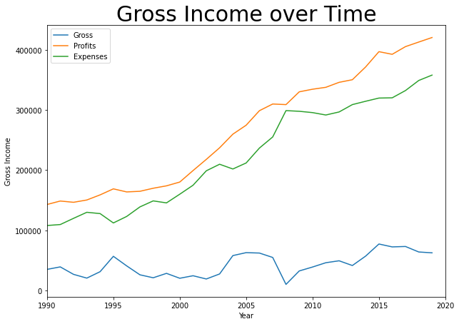
3.6. More Advanced Plotting#
Let’s talk briefly about some other specifications you can do with your graph.
import numpy as np
import matplotlib.pyplot as plt

#Importing the data from the file as we have before. See Yesterdays lecture for the explanations.
year = []
expenses = []
profits = []

with open('finances.txt','r') as infile:

  headers = infile.readline()
  for line in infile:
    data1, data2, data3 = line.split()
    year.append(float(data1))
    expenses.append(float(data2))
    profits.append(float(data3))

expenses = np.array(expenses)
profits = np.array(profits)
gross = profits - expenses

#You can alter the dimensions of the figure with the plt.figure method.
# See the documentation for plt.figure for other specifications you can do.
plt.figure(figsize=(10,7))
#We can plot multiple data sets on the same line by using multiple plt.plot commands.
plt.plot(year, gross, label='Gross')
plt.plot(year, profits, label='Profits')
plt.plot(year, expenses, label = 'Expenses')
#plt.xlim and plt.ylim can set the range that is displayed on the graph.
#Put the bounds inside a tuple: (lowerbound, upperbound)
plt.xlim((1990,2020))
#Add a plot title with plt.title
#Note that we have to put quotes around the title in order to turn it into a string
#We can specify things like font size and location.
plt.title('Gross Income over Time',fontsize=30, fontname="Comic Sans MS")
#xlabel and ylable add axis labels.
plt.xlabel('Year')
plt.ylabel('Gross Income')
#If you have added labels to your plotted data in plt.plot, this command can add a legend.
#The location of the legend can also be specified. Check out the documentation for details.
plt.legend()
plt.show()
findfont: Font family ['Comic Sans MS'] not found. Falling back to DejaVu Sans.