6. Day 3#

6.1. Goals/Anti-goals#

Goal: Provide a tour of several different libraries
Goal: Demonstrate the synergy of the “Python Universe”
Goal: Demonstrate paradigm “get idea then translate into code”
Goal: Demonstrate paradigm “write one line, test, then continue”
Anti-goal: Teach specific functions and specific arguments
Anti-goal: Confuse you

6.2. Roadmap#

A) Obtain dataset from the internet

B) Prepare dataset for analysis with pandas

C) Cluster dataset with sklearn

D) Dimensionality reduction with UMAP, visualization with matplotlib

6.3. A) Obtain dataset from the internet#

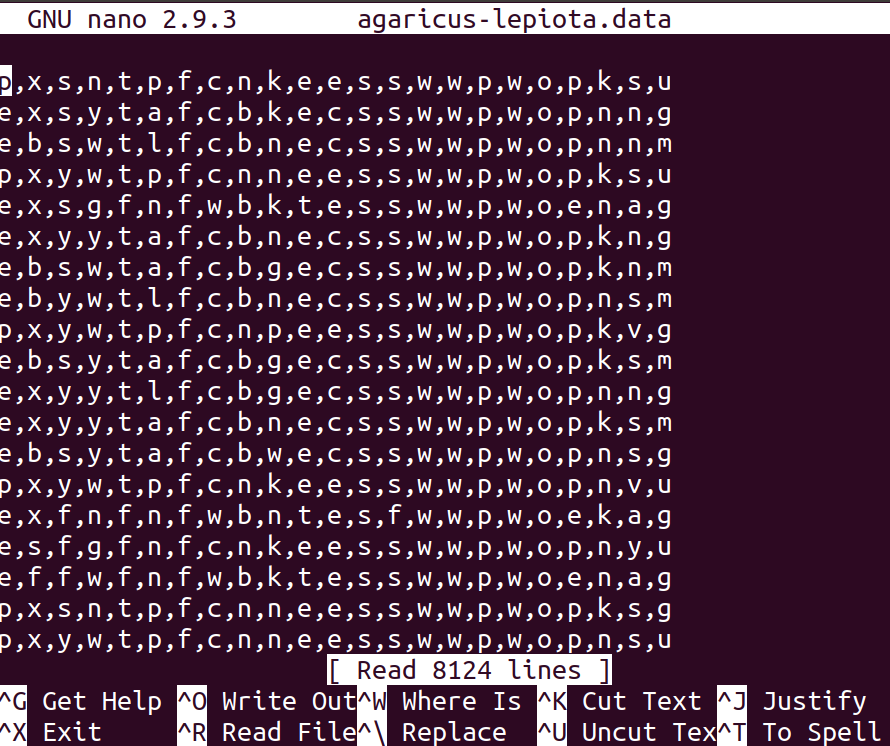
6.3.1. Description:#

23 species
Coincidentally 23 features (columns)
8124 samples (rows)
11th column has missing data

6.3.2. Image of dataset:#

alt text

6.4. B) Prepare dataset for analysis using pandas#

pandas
library in python
perfect for matrix-like data of mixed types (numbers, strings, etc.)

6.4.1. Overall Strategy#

Get dataset into python. Here is the mushroom csv file
Deal with missing data (drop column)
Transform letters into numbers (one-hot encoding)

6.4.2. 0) Get dataset into python#

get pandas library
get a hard coded address for the file
try a simple usage of read_csv
check our work
update our usage of read_csv and check work again

# get library
import pandas as pd

# get a hard coded address for the file
mushroom_dataset_address='../data/agaricus-lepiota.csv'

# try a simple usage of read_csv
my_Panda=pd.read_csv(mushroom_dataset_address)

# check our work
my_Panda

	p	x	s	n	t	p.1	f	c	n.1	k	...	s.2	w	w.1	p.2	w.2	o	p.3	k.1	s.3	u
0	e	x	s	y	t	a	f	c	b	k	...	s	w	w	p	w	o	p	n	n	g
1	e	b	s	w	t	l	f	c	b	n	...	s	w	w	p	w	o	p	n	n	m
2	p	x	y	w	t	p	f	c	n	n	...	s	w	w	p	w	o	p	k	s	u
3	e	x	s	g	f	n	f	w	b	k	...	s	w	w	p	w	o	e	n	a	g
4	e	x	y	y	t	a	f	c	b	n	...	s	w	w	p	w	o	p	k	n	g
...	...	...	...	...	...	...	...	...	...	...	...	...	...	...	...	...	...	...	...	...	...
8118	e	k	s	n	f	n	a	c	b	y	...	s	o	o	p	o	o	p	b	c	l
8119	e	x	s	n	f	n	a	c	b	y	...	s	o	o	p	n	o	p	b	v	l
8120	e	f	s	n	f	n	a	c	b	n	...	s	o	o	p	o	o	p	b	c	l
8121	p	k	y	n	f	y	f	c	n	b	...	k	w	w	p	w	o	e	w	v	l
8122	e	x	s	n	f	n	a	c	b	y	...	s	o	o	p	o	o	p	o	c	l

8123 rows × 23 columns

# update our usage of read_csv and check work again
my_Panda=pd.read_csv(mushroom_dataset_address,header=None)
my_Panda

	0	1	2	3	4	5	6	7	8	9	...	13	14	15	16	17	18	19	20	21	22
0	p	x	s	n	t	p	f	c	n	k	...	s	w	w	p	w	o	p	k	s	u
1	e	x	s	y	t	a	f	c	b	k	...	s	w	w	p	w	o	p	n	n	g
2	e	b	s	w	t	l	f	c	b	n	...	s	w	w	p	w	o	p	n	n	m
3	p	x	y	w	t	p	f	c	n	n	...	s	w	w	p	w	o	p	k	s	u
4	e	x	s	g	f	n	f	w	b	k	...	s	w	w	p	w	o	e	n	a	g
...	...	...	...	...	...	...	...	...	...	...	...	...	...	...	...	...	...	...	...	...	...
8119	e	k	s	n	f	n	a	c	b	y	...	s	o	o	p	o	o	p	b	c	l
8120	e	x	s	n	f	n	a	c	b	y	...	s	o	o	p	n	o	p	b	v	l
8121	e	f	s	n	f	n	a	c	b	n	...	s	o	o	p	o	o	p	b	c	l
8122	p	k	y	n	f	y	f	c	n	b	...	k	w	w	p	w	o	e	w	v	l
8123	e	x	s	n	f	n	a	c	b	y	...	s	o	o	p	o	o	p	o	c	l

8124 rows × 23 columns

6.4.3. 1) Deal with missing data (drop column)#

We need a fast and clear approach

use the function DataFrame.drop
check our work

# use the function DataFrame.drop
## labels indicates the "name" of the column to drop
## axis indicates whether we are dropping from columns or rows (10 exists on both)
## inplace means that we are modifying the variable my_Panda instead of getting a result returned
my_Panda_column_dropped=my_Panda.drop(labels=11,axis='columns')

# check our work
my_Panda_column_dropped

	0	1	2	3	4	5	6	7	8	9	...	13	14	15	16	17	18	19	20	21	22
0	p	x	s	n	t	p	f	c	n	k	...	s	w	w	p	w	o	p	k	s	u
1	e	x	s	y	t	a	f	c	b	k	...	s	w	w	p	w	o	p	n	n	g
2	e	b	s	w	t	l	f	c	b	n	...	s	w	w	p	w	o	p	n	n	m
3	p	x	y	w	t	p	f	c	n	n	...	s	w	w	p	w	o	p	k	s	u
4	e	x	s	g	f	n	f	w	b	k	...	s	w	w	p	w	o	e	n	a	g
...	...	...	...	...	...	...	...	...	...	...	...	...	...	...	...	...	...	...	...	...	...
8119	e	k	s	n	f	n	a	c	b	y	...	s	o	o	p	o	o	p	b	c	l
8120	e	x	s	n	f	n	a	c	b	y	...	s	o	o	p	n	o	p	b	v	l
8121	e	f	s	n	f	n	a	c	b	n	...	s	o	o	p	o	o	p	b	c	l
8122	p	k	y	n	f	y	f	c	n	b	...	k	w	w	p	w	o	e	w	v	l
8123	e	x	s	n	f	n	a	c	b	y	...	s	o	o	p	o	o	p	o	c	l

8124 rows × 22 columns

6.4.4. 2) Transform letters into numbers#

Why?

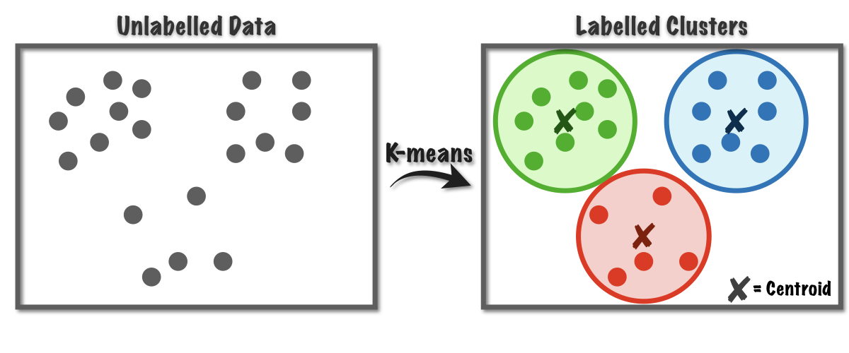
6.4.4.1. Background: clustering#

8,124 samples -> which samples come from the same species?

Clustering: Group datapoints based on location

6.4.4.2. Image#

source:: https://miro.medium.com/max/1200/1*rw8IUza1dbffBhiA4i0GNQ.png

alt text

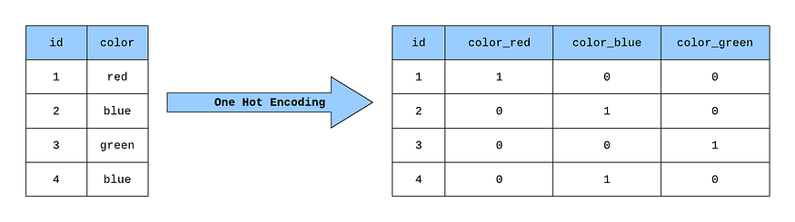
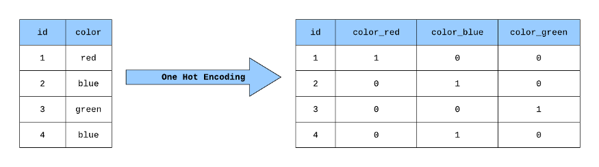
6.4.4.3. One-hot encoding#

To cluster, we need to put data points in spatial locations

Right now each datapoint has 23 letters

We use the strategy of “one-hot encoding”

6.4.4.4. image#

source: https://miro.medium.com/max/875/1*ggtP4a5YaRx6l09KQaYOnw.png

alt text

6.4.4.5. Code#

# one hot encoding
## this time, we got a copy of the dataset back instead of operating on the variable my_Panda directly
## we specify what to encode using 'data'
## we provide a list of columns using my_Panda.columns - we could have also type the list [0,1,2,...,20,21,22]
my_Panda_dummies=pd.get_dummies(data=my_Panda_column_dropped,columns=my_Panda_column_dropped.columns)

# check our work
my_Panda_dummies

	0_e	0_p	1_b	1_c	1_f	1_k	1_s	1_x	2_f	2_g	...	21_s	21_v	21_y	22_d	22_g	22_l	22_m	22_p	22_u	22_w
0	0	1	0	0	0	0	0	1	0	0	...	1	0	0	0	0	0	0	0	1	0
1	1	0	0	0	0	0	0	1	0	0	...	0	0	0	0	1	0	0	0	0	0
2	1	0	1	0	0	0	0	0	0	0	...	0	0	0	0	0	0	1	0	0	0
3	0	1	0	0	0	0	0	1	0	0	...	1	0	0	0	0	0	0	0	1	0
4	1	0	0	0	0	0	0	1	0	0	...	0	0	0	0	1	0	0	0	0	0
...	...	...	...	...	...	...	...	...	...	...	...	...	...	...	...	...	...	...	...	...	...
8119	1	0	0	0	0	1	0	0	0	0	...	0	0	0	0	0	1	0	0	0	0
8120	1	0	0	0	0	0	0	1	0	0	...	0	1	0	0	0	1	0	0	0	0
8121	1	0	0	0	1	0	0	0	0	0	...	0	0	0	0	0	1	0	0	0	0
8122	0	1	0	0	0	1	0	0	0	0	...	0	1	0	0	0	1	0	0	0	0
8123	1	0	0	0	0	0	0	1	0	0	...	0	0	0	0	0	1	0	0	0	0

8124 rows × 114 columns

6.5. C) Cluster the data with sklearn#

6.5.1. Background:#

In the above image, data had 2 dimensions so we could visually assess clustering

For n-dimensional case We turn to a clustering algorithm.

Within sklearn we choose the algorithm K-means.

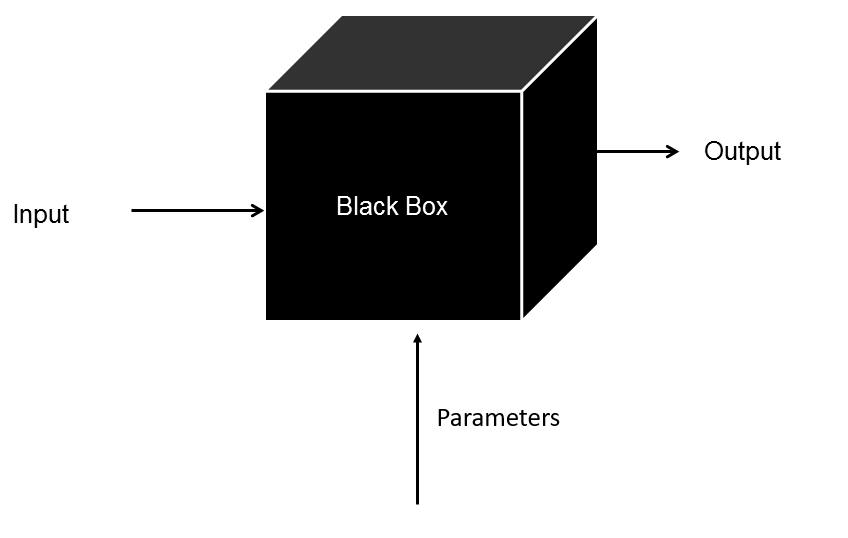
Because time constraints we treat KMeans like a black box

6.5.1.1. Image: Black box#

Black box: give input, get output, dont ask how

Step 1)

Parameters: arguments that our chosen algorithm requires

Step 2)

Input: my_Panda_dummies
Output: list of labels

alt text

6.5.1.2. Giving parameters to K-means black box#

KMeans requires the number of clusters (23)

from sklearn.cluster import KMeans

#declare our black box by calling KMeans
##we give the black box/calculator the name my_KMeans_tool
my_KMeans_tool=KMeans(n_clusters=23)

print(my_KMeans_tool)

KMeans(n_clusters=23)

#we havent told my_KMeans_tool about our data yet, so we expect this to fail
print(my_KMeans_tool.labels_)

---------------------------------------------------------------------------
AttributeError                            Traceback (most recent call last)
<ipython-input-13-9d53e9cea4d7> in <module>
      1 #we havent told my_KMeans_tool about our data yet, so we expect this to fail
----> 2 print(my_KMeans_tool.labels_)

AttributeError: 'KMeans' object has no attribute 'labels_'

6.5.1.3. Black Box Operation#

sklearn (often) relies on the function “fit_transform” to connect the data with the algorithm

#tell my_KMeans_tool about our data
## we ignore the output
## notice how sklearn's KMeans flawlessly accepts a panda as input
my_KMeans_tool.fit_transform(X=my_Panda_dummies)

array([[3.77102947, 4.54519275, 4.26060768, ..., 3.7859389 , 3.64273399,
        5.07033858],
       [3.58657502, 5.01968512, 3.73980095, ..., 3.05505046, 3.88277768,
        4.85197554],
       [3.44952673, 5.08565682, 3.87835876, ..., 3.41565026, 3.96295279,
        5.11940752],
       ...,
       [4.51655119, 5.20279094, 4.51386752, ..., 4.65474668, 4.1459457 ,
        5.16801058],
       [4.4688548 , 2.70655571, 4.72434593, ..., 4.61880215, 3.59594233,
        4.76532615],
       [4.59105719, 5.20279094, 4.44565956, ..., 4.72581563, 4.1672875 ,
        5.26387057]])

#now we see that we have the labels that expected
print(my_KMeans_tool.labels_)
print(len(my_KMeans_tool.labels_))

[ 4 11 11 ... 10  8 10]
8124

6.5.1.4. Done?#

Got a label for every data point.

Philosophical viewpoint: We did perfectly, the algorithm worked exactly as intended

Are our clusters meaningful?

Hard to say. We could try to relate our clusters to some external dataset. We don’t have that here.

Lets try a visualization.

In our case, we are going to:

Take our 114 dimensional dataset (114 columns)
Reduce the dimensionality to 2.
Plot all datapoints, getting (x,y) from dimensionality reduction and colors from clustering label.

If each color of datapoints is separated from every other cluster, then we have some assurance that our dataset is “robustly clusterable”. That’s it.

6.6. Dimensionality Reduction and Visualization#

6.6.1. Naive approach:#

choose two columns and drop all of the rest

6.6.2. Which algorithm?#

PCA, PLS-DA, t-SNE, UMAP

demonstrate the bredth/synergy of the python language, so we choose UMAP (not in sklearn)

Even though UMAP is not in sklearn, the authors of UMAP wrote it in such a way that it “works like” sklearn functions.

6.6.3. Strategy#

create our UMAP black box
operate that black box on our dataset
obtain a 2-d coordinate pair for every datapoint
plot those pairs, with the color of the datapoint reflecting the clustering label from KMeans

6.6.4. Code#

# create our black box
## import our library
import umap

## declare a couple of parameters that we wont get into
n_neighbors=10
min_dist=0.1
n_components=2
metric='euclidean'


##just like last time, we declare a "UMAP calculator" and send a couple of parameters
my_UMAP=umap.UMAP(n_neighbors=n_neighbors,min_dist=min_dist,n_components=n_components,metric=metric)

print(my_UMAP)

UMAP(dens_frac=0.0, dens_lambda=0.0, n_neighbors=10)

# again, we use fit transform to inform our calculator of our dataset 
## again, notice how it flawlessly accepts a panda
## this time, we actually want the thing that gets spit back out
my_UMAP.fit_transform(my_Panda_dummies)

array([[ -7.6440673 , -12.353603  ],
       [ -0.26427558,   8.624089  ],
       [ -0.47456995,   7.971237  ],
       ...,
       [ 11.546015  ,  -6.2244453 ],
       [ 19.653965  ,   8.905327  ],
       [ 11.451685  ,  -6.2179003 ]], dtype=float32)

We redo to capture the 2D coordinate list

# 2) and 3)
my_numpy_2d=my_UMAP.fit_transform(my_Panda_dummies)
print(len(my_numpy_2d))

import matplotlib.pyplot as plt

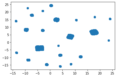
#4)
#scatter plot takes
#list of x coordinates
#list of y coordinates
plt.scatter(
    my_numpy_2d[:,0],
    my_numpy_2d[:,1]
)
plt.show()

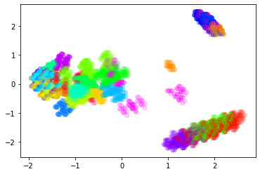
#4) redo with arguments to make the color in accordance wiht the KMeans cluster labels



#an opacity parameter
plt.scatter(
    my_numpy_2d[:,0],
    my_numpy_2d[:,1],
    #a label list
    c=my_KMeans_tool.labels_,
    #a color bar (literally the rainbox)
    cmap='gist_rainbow',
    #make the points mildly transparent so we can see generalities
    alpha=0.2
)
plt.show()

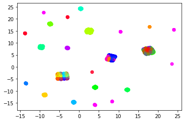
6.6.5. Observations#

Our dimensionality reduction technique independently produced 23 visually-discernible clusters, but those clusters only partially agree with the KMeans clustering

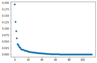
6.6.6. Bonus: Dim Reduction with PCA#

import matplotlib.pyplot as plt
from sklearn.decomposition import PCA
my_PCA=PCA()
my_PCAd_coordinates=my_PCA.fit_transform(my_Panda_dummies)
plt.scatter(range(len(my_PCA.explained_variance_ratio_)),my_PCA.explained_variance_ratio_)
plt.show()
print(my_PCAd_coordinates.shape)
print(my_PCAd_coordinates[:,0].shape)
plt.scatter(my_PCAd_coordinates[:,0],my_PCAd_coordinates[:,1],c=my_KMeans_tool.labels_,cmap='gist_rainbow',alpha=0.2)
plt.show()

(8124, 114)
(8124,)

Python Intensive Training

Day 3

Contents

6. Day 3#

6.1. Goals/Anti-goals#

6.2. Roadmap#

6.3. A) Obtain dataset from the internet#

6.3.1. Description:#

6.3.2. Image of dataset:#

6.4. B) Prepare dataset for analysis using pandas#

6.4.1. Overall Strategy#

6.4.2. 0) Get dataset into python#

6.4.3. 1) Deal with missing data (drop column)#

6.4.4. 2) Transform letters into numbers#

6.4.4.1. Background: clustering#

6.4.4.2. Image#

6.4.4.3. One-hot encoding#

6.4.4.4. image#

6.4.4.5. Code#

6.5. C) Cluster the data with sklearn#

6.5.1. Background:#

6.5.1.1. Image: Black box#

6.5.1.2. Giving parameters to K-means black box#

6.5.1.3. Black Box Operation#

6.5.1.4. Done?#

6.6. Dimensionality Reduction and Visualization#

6.6.1. Naive approach:#

6.6.2. Which algorithm?#

6.6.3. Strategy#

6.6.4. Code#

6.6.5. Observations#

6.6.6. Bonus: Dim Reduction with PCA#