2 Example data: COVID-19 counts

Before getting into how to split the data into training and validation parts, let’s get to know the examples that we’ll be working through today. First, though, we need to load some packages and set the path to use for loading data.

# import libraries
library( "dplyr" )
library( "lubridate" )
library( "readr" )
library( "gbm" )
library( "tidymodels")
library( "remotes" )

# import the covid data set
covid = read_csv( "https://raw.githubusercontent.com/ucdavisdatalab/workshop-model-validation/master/data/covid.csv" )

The data sets that we’ll use for illustration are a time series of daily hospital admissions for COVID-19, and a time series of the number of beds occupied overnight by COVID-19 patients. Our goal is to create models that can predict the future values of these time series. Let’s take a look at the time series. In the code that follows, you’ll see the with() function, which tells R where to check first for data when it encounters a variable name. That makes the code cleaner to read and write, as there are fewer repetitions of the prefix covid$ to access data.

# layout the plot window for side-by-side figures
layout( matrix(1:2, 1, 2))

# plot the admissions time series
with( covid, plot(date, COVID_NEW_ADM_CNT, type='l') )

# plot the overnight census time series
with( covid, plot(date, COVID_PT_CNT_M, type='l') )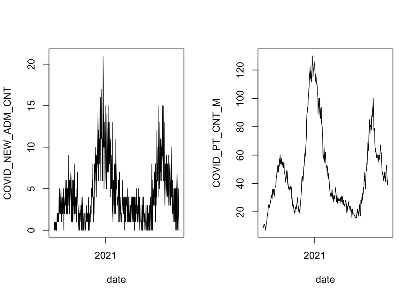

That’s the daily number of new admissions on the left (the variable comes out of the hospital’s records system as COVID_NEW_ADM_CNT), and the number of beds occupied overnight by COVID-19 patients on the right (this variable is coded in the hospital records as COVID_PT_CNT_M, and the hospital refers to the overnight count as the midnight census). The two follow a similar pattern, with cases arriving in waves that rise and fall quickly against a baseline of low counts. There is more noise in the time series of new admissions, while the midnight census is more stable from one day to the next.