2 Tutorial with R
Finally, now we’re going to work in R to get some hands-on practice with the concepts we just discussed.
We’ll be working with sp objects today, but you should also know that there are sf objects as well. Roger Bivand’s review of spatial data for R is helpful for understading the options for working with spatial data.
2.1 Getting Started
2.1.1 Download the data
The data for this workshop is available in the data folder in this repository, or you can download a .zip file from Box.
2.1.2 Start R
Pick the R flavor of your choice - regular R, R Studio, etc. - and start it up. You can either add the commands we’ll be using to a script file to run, or you can just run the lines individually in your console to see how they work. It’s up to you.
2.1.3 Libraries
Let’s load the libraries we’ll need.
TIP: I add to this section as I write my code and need new libraries. Keep them in one place for easy reference.
#install.packages("sf")
#install.packages("terra")

library("sf")
library("terra")
2.1.4 Set your working directory to the folder where you saved your data
TIP: Windows users, use \ instead of or switch the direction of the slashes to /… it has to do with escape characters.
setwd("C:/WorkshopData")Replace C:/Workshops with the path to the folder in which you saved your data. This workshop assumes your workshop materials are in a folder called “workshopData” and the data is in a folder called “data”.
2.2 Vector Data
2.2.1 Read the data into our R session
Because “points” by itself is a command and we don’t want confusion, I’ve added “ws.” (WS for watershed) to the front of my variable names.
Most of the vector data formats can be read into r with the st_read function. To see the help files for this function, run ?st_read in your console.
ws.points<-st_read("data/WBDHU8_Points_SF.geojson")## Reading layer `WBDHU8_Points_SF' from data source `C:\Users\mmtobias\Documents\GitHub\datalab\workshop_coordinate_reference_systems\data\WBDHU8_Points_SF.geojson' using driver `GeoJSON'
## Simple feature collection with 6 features and 15 fields
## Geometry type: POINT
## Dimension: XY
## Bounding box: xmin: -250560.3 ymin: -81326.09 xmax: -162308 ymax: 21467.35
## Projected CRS: NAD83 / California Albersws.polygons<-st_read("data/WBDHU8_SF.geojson")## Reading layer `WBDHU8_SF' from data source `C:\Users\mmtobias\Documents\GitHub\datalab\workshop_coordinate_reference_systems\data\WBDHU8_SF.geojson' using driver `GeoJSON'
## Simple feature collection with 6 features and 10 fields
## Geometry type: MULTIPOLYGON
## Dimension: XY
## Bounding box: xmin: -278890 ymin: -122244.5 xmax: -122332.5 ymax: 75400.89
## Projected CRS: NAD83 / California Albersws.streams<-st_read("data/flowlines.shp")## Reading layer `flowlines' from data source `C:\Users\mmtobias\Documents\GitHub\datalab\workshop_coordinate_reference_systems\data\flowlines.shp' using driver `ESRI Shapefile'
## Simple feature collection with 4857 features and 11 fields
## Geometry type: LINESTRING
## Dimension: XY
## Bounding box: xmin: -265095.9 ymin: -116267.6 xmax: -124022.6 ymax: 72531.26
## CRS: NALet’s look at the contents of one of the files:
ws.polygons## Simple feature collection with 6 features and 10 fields
## Geometry type: MULTIPOLYGON
## Dimension: XY
## Bounding box: xmin: -278890 ymin: -122244.5 xmax: -122332.5 ymax: 75400.89
## Projected CRS: NAD83 / California Albers
## TNMID LOADDATE AREAACRES AREASQKM STATES
## 1 {7A24A43D-27F0-4B35-A273-AF361042B2A8} 2012-06-11 489068.6 1979.19 CA
## 2 {F0F29A9E-E9D6-4F24-9D1A-CB8C7E22141E} 2012-06-11 853256.6 3453.01 CA
## 3 {7E0042D2-0B68-40B4-83FA-2850D989E91A} 2012-06-11 461004.8 1865.62 CA
## 4 {BE7EC116-0BE6-419E-8165-84B063FE8468} 2012-06-11 417511.7 1689.61 CA
## 5 {E67739F5-92F6-49B0-A017-F4A0372DD4F9} 2012-06-11 784983.8 3176.72 CA
## 6 {9B6A9642-9FE9-4F0B-BB30-90E918E63551} 2012-06-11 431362.9 1745.67 CA
## HUC8 NAME SHAPE_LENG SHAPE_AREA Rank_Acres
## 1 18050005 Tomales-Drake Bays 3.177305 0.2031323 4
## 2 18050004 San Francisco Bay 4.019037 0.3522663 6
## 3 18050003 Coyote 3.232746 0.1895257 3
## 4 18050001 Suisun Bay 2.795490 0.1735314 1
## 5 18050002 San Pablo Bay 3.985180 0.3266645 5
## 6 18050006 San Francisco Coastal South 2.743098 0.1774121 2
## geometry
## 1 MULTIPOLYGON (((-252626.2 4...
## 2 MULTIPOLYGON (((-187360.2 -...
## 3 MULTIPOLYGON (((-164610.2 -...
## 4 MULTIPOLYGON (((-188614.2 4...
## 5 MULTIPOLYGON (((-227456.2 7...
## 6 MULTIPOLYGON (((-220773.4 -...Note that the output not only shows the data but gives you some metadata as well, such as the geometry type, bounding box (bbox), and the projected CRS, which is “NAD83 / California Albers”.
2.2.2 Indentifying the Assigned CRS
To see just the coordinate reference system, we can use the crs() command. Let’s check the CRS for each of our files:
st_crs(ws.points)## Coordinate Reference System:
## User input: NAD83 / California Albers
## wkt:
## PROJCRS["NAD83 / California Albers",
## BASEGEOGCRS["NAD83",
## DATUM["North American Datum 1983",
## ELLIPSOID["GRS 1980",6378137,298.257222101,
## LENGTHUNIT["metre",1]]],
## PRIMEM["Greenwich",0,
## ANGLEUNIT["degree",0.0174532925199433]],
## ID["EPSG",4269]],
## CONVERSION["California Albers",
## METHOD["Albers Equal Area",
## ID["EPSG",9822]],
## PARAMETER["Latitude of false origin",0,
## ANGLEUNIT["degree",0.0174532925199433],
## ID["EPSG",8821]],
## PARAMETER["Longitude of false origin",-120,
## ANGLEUNIT["degree",0.0174532925199433],
## ID["EPSG",8822]],
## PARAMETER["Latitude of 1st standard parallel",34,
## ANGLEUNIT["degree",0.0174532925199433],
## ID["EPSG",8823]],
## PARAMETER["Latitude of 2nd standard parallel",40.5,
## ANGLEUNIT["degree",0.0174532925199433],
## ID["EPSG",8824]],
## PARAMETER["Easting at false origin",0,
## LENGTHUNIT["metre",1],
## ID["EPSG",8826]],
## PARAMETER["Northing at false origin",-4000000,
## LENGTHUNIT["metre",1],
## ID["EPSG",8827]]],
## CS[Cartesian,2],
## AXIS["easting (X)",east,
## ORDER[1],
## LENGTHUNIT["metre",1]],
## AXIS["northing (Y)",north,
## ORDER[2],
## LENGTHUNIT["metre",1]],
## USAGE[
## SCOPE["State-wide spatial data management."],
## AREA["United States (USA) - California."],
## BBOX[32.53,-124.45,42.01,-114.12]],
## ID["EPSG",3310]]st_crs(ws.polygons)## Coordinate Reference System:
## User input: NAD83 / California Albers
## wkt:
## PROJCRS["NAD83 / California Albers",
## BASEGEOGCRS["NAD83",
## DATUM["North American Datum 1983",
## ELLIPSOID["GRS 1980",6378137,298.257222101,
## LENGTHUNIT["metre",1]]],
## PRIMEM["Greenwich",0,
## ANGLEUNIT["degree",0.0174532925199433]],
## ID["EPSG",4269]],
## CONVERSION["California Albers",
## METHOD["Albers Equal Area",
## ID["EPSG",9822]],
## PARAMETER["Latitude of false origin",0,
## ANGLEUNIT["degree",0.0174532925199433],
## ID["EPSG",8821]],
## PARAMETER["Longitude of false origin",-120,
## ANGLEUNIT["degree",0.0174532925199433],
## ID["EPSG",8822]],
## PARAMETER["Latitude of 1st standard parallel",34,
## ANGLEUNIT["degree",0.0174532925199433],
## ID["EPSG",8823]],
## PARAMETER["Latitude of 2nd standard parallel",40.5,
## ANGLEUNIT["degree",0.0174532925199433],
## ID["EPSG",8824]],
## PARAMETER["Easting at false origin",0,
## LENGTHUNIT["metre",1],
## ID["EPSG",8826]],
## PARAMETER["Northing at false origin",-4000000,
## LENGTHUNIT["metre",1],
## ID["EPSG",8827]]],
## CS[Cartesian,2],
## AXIS["easting (X)",east,
## ORDER[1],
## LENGTHUNIT["metre",1]],
## AXIS["northing (Y)",north,
## ORDER[2],
## LENGTHUNIT["metre",1]],
## USAGE[
## SCOPE["State-wide spatial data management."],
## AREA["United States (USA) - California."],
## BBOX[32.53,-124.45,42.01,-114.12]],
## ID["EPSG",3310]]st_crs(ws.streams)## Coordinate Reference System: NAIt looks like the streams dataset does not have its CRS defined.
2.2.3 Defining a CRS
Let’s be clear that the streams data has a CRS, but R doesn’t know what it should be. (Someone may have forgotten to include the .prj file in this shapefile.) You don’t get to decide what you want it to be, but rather figure out what it IS and tell R which coordinate system to use. How do you know which CRS the data has if its not properly defined? Typically, you first ask the person who sent it. If that fails, you can search for another version of the data online to get a file with the correct projection information. Finally, outright guessing can work, but isn’t recommended. We know that the CRS for this data should be EPSG 3309 (because that’s what the instructor saved it as before she deleted the .prj file… shapefiles are not a great exchange format, FYI).
Set the CRS:
ws.streams.3309<-st_set_crs(ws.streams, value=3309) EPSG 3309 = California Albers, NAD 27
Let’s imagine we loaded up our data and find that it shows up on a map in the wrong location. What happened? Someone defined the CRS incorrectly. How do you fix it? First you figure out what the CRS should be, then you run one of the lines above with the correct CRS definition to fix the file.
2.2.4 Tranforming / Reprojecting Vector Data
We need to get all our data into the same projection so it will plot together on one map before we can do any kind of spatial process on the data.
# tranform/reproject vector data
ws.streams.3310<-st_transform(ws.streams.3309, crs=3310)

#   another option: match the CRS of the polygons data
ws.streams.3310<-st_transform(ws.streams.3309, crs=st_crs(ws.polygons))
Let’s check the CRS for each of our files again:
st_crs(ws.points)## Coordinate Reference System:
## User input: NAD83 / California Albers
## wkt:
## PROJCRS["NAD83 / California Albers",
## BASEGEOGCRS["NAD83",
## DATUM["North American Datum 1983",
## ELLIPSOID["GRS 1980",6378137,298.257222101,
## LENGTHUNIT["metre",1]]],
## PRIMEM["Greenwich",0,
## ANGLEUNIT["degree",0.0174532925199433]],
## ID["EPSG",4269]],
## CONVERSION["California Albers",
## METHOD["Albers Equal Area",
## ID["EPSG",9822]],
## PARAMETER["Latitude of false origin",0,
## ANGLEUNIT["degree",0.0174532925199433],
## ID["EPSG",8821]],
## PARAMETER["Longitude of false origin",-120,
## ANGLEUNIT["degree",0.0174532925199433],
## ID["EPSG",8822]],
## PARAMETER["Latitude of 1st standard parallel",34,
## ANGLEUNIT["degree",0.0174532925199433],
## ID["EPSG",8823]],
## PARAMETER["Latitude of 2nd standard parallel",40.5,
## ANGLEUNIT["degree",0.0174532925199433],
## ID["EPSG",8824]],
## PARAMETER["Easting at false origin",0,
## LENGTHUNIT["metre",1],
## ID["EPSG",8826]],
## PARAMETER["Northing at false origin",-4000000,
## LENGTHUNIT["metre",1],
## ID["EPSG",8827]]],
## CS[Cartesian,2],
## AXIS["easting (X)",east,
## ORDER[1],
## LENGTHUNIT["metre",1]],
## AXIS["northing (Y)",north,
## ORDER[2],
## LENGTHUNIT["metre",1]],
## USAGE[
## SCOPE["State-wide spatial data management."],
## AREA["United States (USA) - California."],
## BBOX[32.53,-124.45,42.01,-114.12]],
## ID["EPSG",3310]]st_crs(ws.polygons)## Coordinate Reference System:
## User input: NAD83 / California Albers
## wkt:
## PROJCRS["NAD83 / California Albers",
## BASEGEOGCRS["NAD83",
## DATUM["North American Datum 1983",
## ELLIPSOID["GRS 1980",6378137,298.257222101,
## LENGTHUNIT["metre",1]]],
## PRIMEM["Greenwich",0,
## ANGLEUNIT["degree",0.0174532925199433]],
## ID["EPSG",4269]],
## CONVERSION["California Albers",
## METHOD["Albers Equal Area",
## ID["EPSG",9822]],
## PARAMETER["Latitude of false origin",0,
## ANGLEUNIT["degree",0.0174532925199433],
## ID["EPSG",8821]],
## PARAMETER["Longitude of false origin",-120,
## ANGLEUNIT["degree",0.0174532925199433],
## ID["EPSG",8822]],
## PARAMETER["Latitude of 1st standard parallel",34,
## ANGLEUNIT["degree",0.0174532925199433],
## ID["EPSG",8823]],
## PARAMETER["Latitude of 2nd standard parallel",40.5,
## ANGLEUNIT["degree",0.0174532925199433],
## ID["EPSG",8824]],
## PARAMETER["Easting at false origin",0,
## LENGTHUNIT["metre",1],
## ID["EPSG",8826]],
## PARAMETER["Northing at false origin",-4000000,
## LENGTHUNIT["metre",1],
## ID["EPSG",8827]]],
## CS[Cartesian,2],
## AXIS["easting (X)",east,
## ORDER[1],
## LENGTHUNIT["metre",1]],
## AXIS["northing (Y)",north,
## ORDER[2],
## LENGTHUNIT["metre",1]],
## USAGE[
## SCOPE["State-wide spatial data management."],
## AREA["United States (USA) - California."],
## BBOX[32.53,-124.45,42.01,-114.12]],
## ID["EPSG",3310]]st_crs(ws.streams)## Coordinate Reference System: NANow they all should match.
2.2.5 Plotting the Data
Lets make a map now that all our data is in the same projection. What if we had tried to do this earlier before we fixed out projection definitions and transformed the files into the same projections?
Load up the CA Counties layer to use as reference in a map:
ca.counties<-st_read("data/CA_Counties.geojson")## Reading layer `CA_Counties' from data source `C:\Users\mmtobias\Documents\GitHub\datalab\workshop_coordinate_reference_systems\data\CA_Counties.geojson' using driver `GeoJSON'
## Simple feature collection with 179 features and 12 fields
## Geometry type: POLYGON
## Dimension: XY
## Bounding box: xmin: -374443.2 ymin: -604504.7 xmax: 540082.8 ymax: 450029.9
## Projected CRS: NAD83 / California AlbersLet’s plot all the data together:
plot(
ca.counties$geometry,
col="#FFFDEA",
border="gray",
xlim=st_bbox(ws.polygons)[1:2],
ylim=st_bbox(ws.polygons)[3:4],
bg="#dff9fd",
main = "Perennial Streams",
sub = "in the San Francisco Bay Watersheds"
)
plot(ws.streams$geometry, col="#3182bd", lwd=1.75, add=TRUE)
plot(ws.points$geometry, col="black", pch=20, cex=3, add=TRUE)
plot(ws.polygons$geometry, lwd=2, border="grey35", add=TRUE)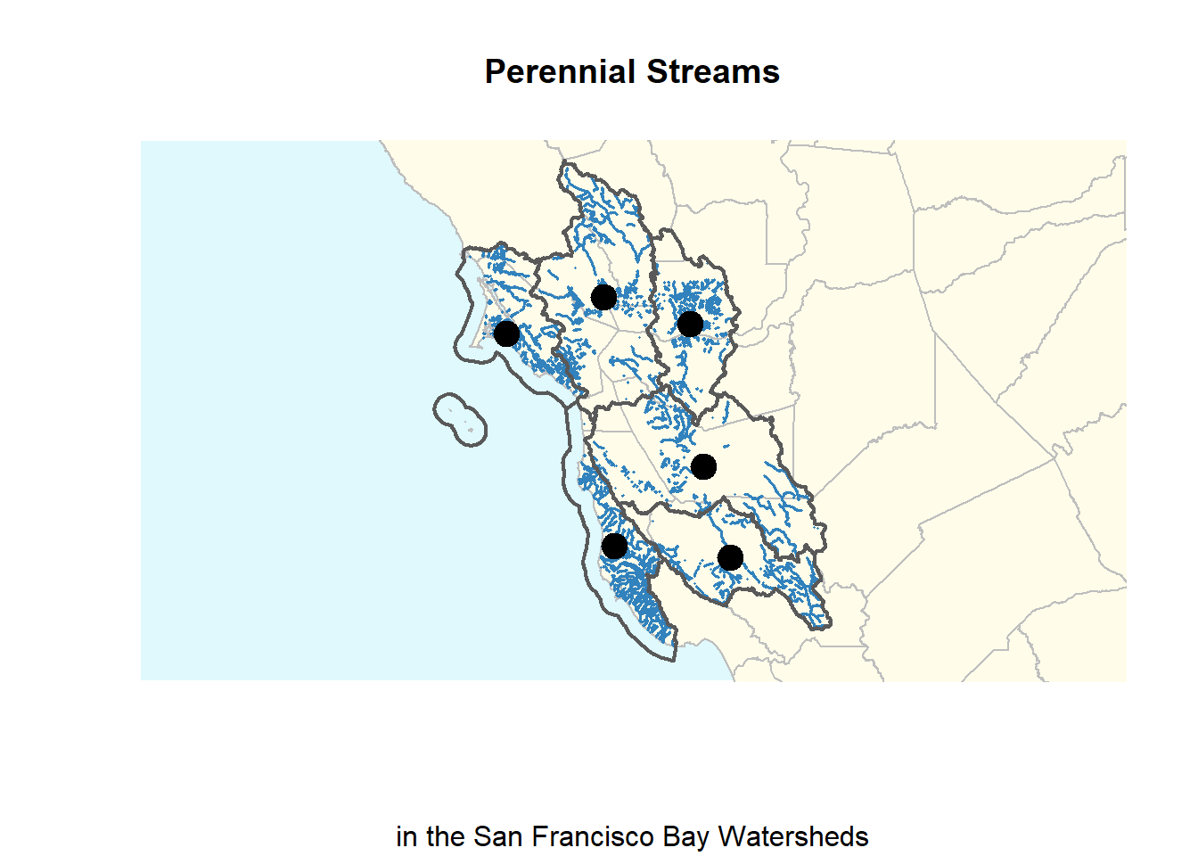 Some explanation of the code above for plotting the spatial data:
*
Some explanation of the code above for plotting the spatial data:
* xlim/ylim sets the extent. Here I used the numbers from the bounding box of the polygon dataset, but you could put in numbers - remember that this is projected data so lat/long won’t work
* add=TRUE makes the 2nd, 3rd, 4th, etc. datasets plot on the same map as the first dataset you plot - order matters
* col sets the fill color for the geometry
* border sets the outline color (or stroke for users of vector graphics programs)
* bg sets the background color for the plot
* colors can be specified with words like “gray” or html hex codes like #dff9fd
2.3 Raster Data
We’ve just looked at how to work with the CRS of vector data. Now let’s look at raster data.
First, we need to install the package that works with raster data. Today we’ll use terra but there are other packages like raster that also work in similar ways.
2.3.1 Load Data
Now we’ll load our data. This is a digital elevation model (DEM) of the City of San Francisco.
dem<-rast(x="data/DEM_SF.tif")2.3.2 Indentifying the Assigned CRS
What is the CRS of this dataset? Note that the command to read the CRS in the terra package is different from sf.
crs(dem)## [1] "GEOGCRS[\"NAD83\",\n DATUM[\"North American Datum 1983\",\n ELLIPSOID[\"GRS 1980\",6378137,298.257222101004,\n LENGTHUNIT[\"metre\",1]]],\n PRIMEM[\"Greenwich\",0,\n ANGLEUNIT[\"degree\",0.0174532925199433]],\n CS[ellipsoidal,2],\n AXIS[\"geodetic latitude (Lat)\",north,\n ORDER[1],\n ANGLEUNIT[\"degree\",0.0174532925199433]],\n AXIS[\"geodetic longitude (Lon)\",east,\n ORDER[2],\n ANGLEUNIT[\"degree\",0.0174532925199433]],\n ID[\"EPSG\",4269]]"2.3.3 Defining a CRS
Our data came with a CRS, but in the event that we needed to define it, we would do it like this:
crs(dem)<-"epsg:4269"2.3.4 Tranforming / Reprojecting Raster Data
So we know that our data is in the CRS with EPSG code 4269. That’s not the same CRS as our other data, so we’ll need to transform it. Again, terra uses different names than sf does. Is this confusing? Yes it is. This is why we read the documentation.
dem.3310<-project(dem, "epsg:3310")2.3.5 Plotting the Data
Now that all of our datasets are in the same projection, we can use them together. Let’s make a map with both our raster and vector data.
plot(dem.3310, col=terrain.colors(50), axes = FALSE, legend = FALSE)
plot(ws.streams.3310$geometry, col="#3182bd", lwd=3, add=TRUE)
plot(ws.polygons$geometry, lwd=1, border="grey35", add=TRUE)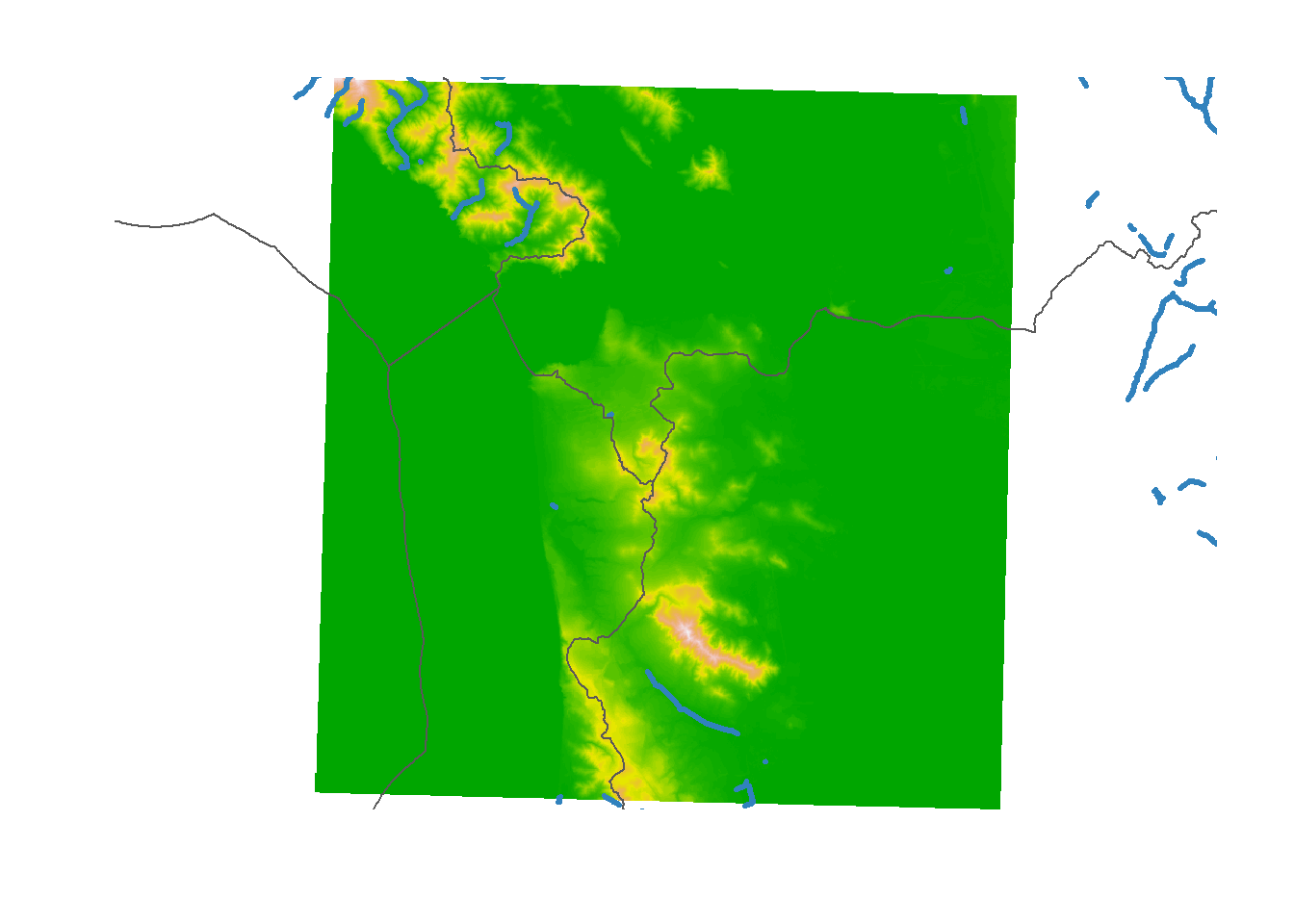
2.4 Conclusion
After completing this workshop, you should now have a better understanding of Coordinate Reference Systems (CRS) or projections, as they are often called colloquially. You can now find out what the CRS is for a dataset and know the common formats this can take. You should understand the difference between defining a CRS and tranforming a dataset (often called “reprojecting” in other GIS programs), when to use them, and how to execute both commands. You’ve also seen how to use the basic plot() function to make a map.
Now that you’ve had some hands-on experience with projections and spatial data, it’s a good time to go back an review the concepts introduced in the beginning of the workshop. You may find that some of it makes more sense now that you have more experience.
Do you now feel like you know everything you need to know and will never have any more questions? Of course not! It’s a learning process that will continue for the rest of your career working with spatial data. Need more help? See data.ucdavis.edu for how to contact your friendly UC Davis GIS Data Curator.
2.5 Resources Used to Compile this Tutorial:
- Geocomputation with R by Robin Lovelace
- Rspatial.org
- Data Carpentry Intro to Geospatial Data with R
- University of Colorado’s Map Projections
- International Institute for Geo-Information Science and Earth Observation (ITC)
- Carlos Furuti’s Projections Page
- ESRI Resource Center - Projections
Map Projection Fun:
- xkcd’s Map Projections
- Jason Davies’ Map Projection Transitions
- Carlos Furuti’s Printable Projections Global projections you can print and assemble