3. Linear Regression

We can use deep learning to estimate a linear regression model.

Begin by importing the necessary packages.

import sklearn
from sklearn import datasets
from sklearn.model_selection import train_test_split
from sklearn.linear_model import LinearRegression
import torch
import seaborn as sns
import matplotlib.pyplot as plt
import pandas as pd

import statsmodels.api as sm
import statsmodels.formula.api as smf

import torchinfo

3.1. Import the data

This example uses data on the progression of diabetes in 442 people with the disease. The inputs are medical variables that were measured in a physical exam: age; sex; blood pressure; body mass index (BMI); blood glucose; LDL, HDL, and total cholesterol. The measurement of disease progression is unitless and based on an unknown calculation. The data is built into the sklearn package’s datasets module.

The predictor variables have already been centered and scaled, so they have mean zero and unit standard deviation. The measure of diabetes has not been centered or scaled.

# import the diabetes dataset
diabetes = datasets.load_diabetes()

print(diabetes.DESCR)

# convert the data to a pandas dataframe
df = pd.DataFrame(diabetes.data, columns=diabetes.feature_names)
df['target'] = diabetes.target

# plot the combinations of variables
sns.pairplot(df)

.. _diabetes_dataset:

Diabetes dataset
----------------

Ten baseline variables, age, sex, body mass index, average blood
pressure, and six blood serum measurements were obtained for each of n =
442 diabetes patients, as well as the response of interest, a
quantitative measure of disease progression one year after baseline.

**Data Set Characteristics:**

:Number of Instances: 442

:Number of Attributes: First 10 columns are numeric predictive values

:Target: Column 11 is a quantitative measure of disease progression one year after baseline

:Attribute Information:
    - age     age in years
    - sex
    - bmi     body mass index
    - bp      average blood pressure
    - s1      tc, total serum cholesterol
    - s2      ldl, low-density lipoproteins
    - s3      hdl, high-density lipoproteins
    - s4      tch, total cholesterol / HDL
    - s5      ltg, possibly log of serum triglycerides level
    - s6      glu, blood sugar level

Note: Each of these 10 feature variables have been mean centered and scaled by the standard deviation times the square root of `n_samples` (i.e. the sum of squares of each column totals 1).

Source URL:
https://www4.stat.ncsu.edu/~boos/var.select/diabetes.html

For more information see:
Bradley Efron, Trevor Hastie, Iain Johnstone and Robert Tibshirani (2004) "Least Angle Regression," Annals of Statistics (with discussion), 407-499.
(https://web.stanford.edu/~hastie/Papers/LARS/LeastAngle_2002.pdf)

<seaborn.axisgrid.PairGrid at 0x153dfbe90>

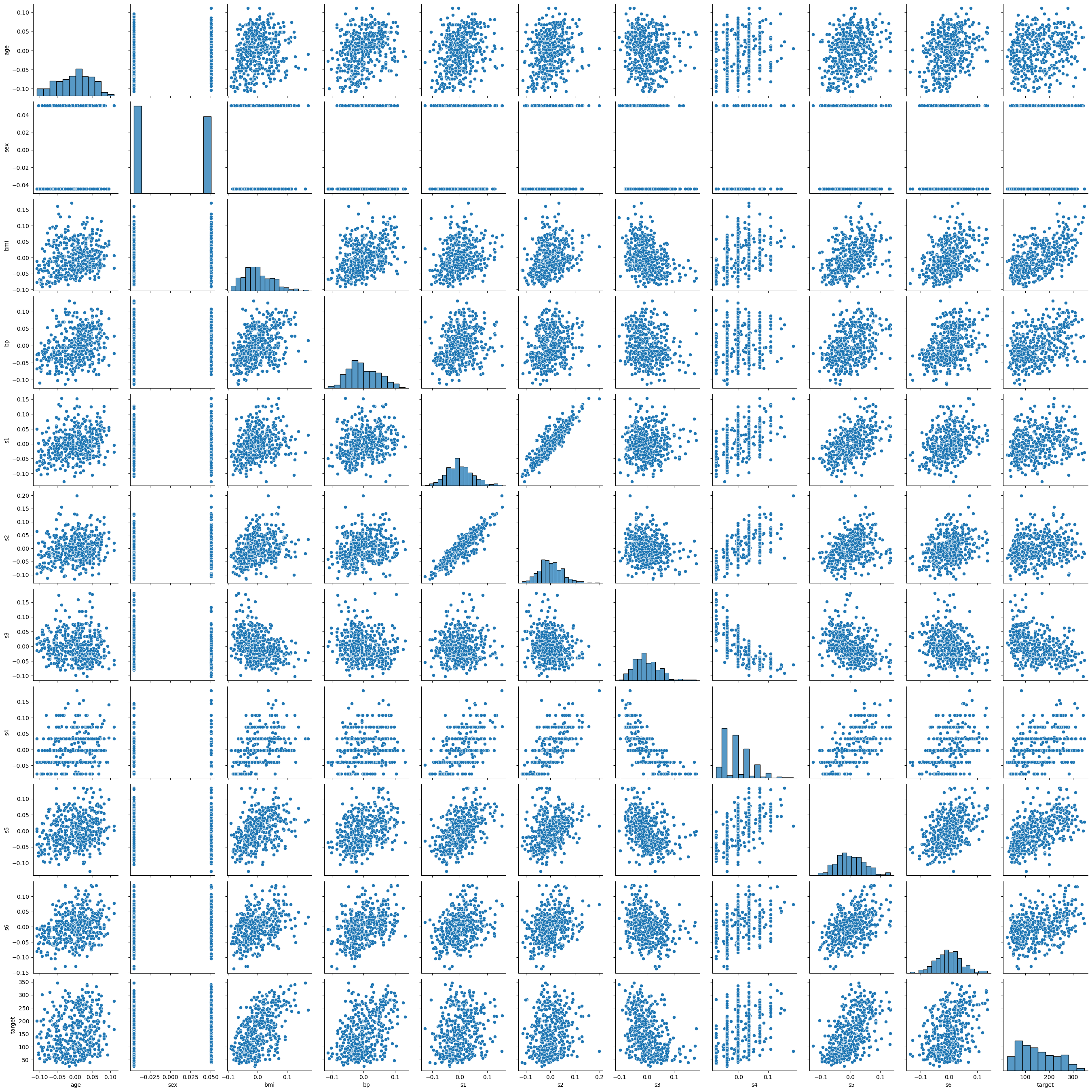
It looks like the target variable is growing with BMI and blood glucose. Let’s create a linear model to examine that.

# create a linear model with BMI and blood glucose.
# estimate the model
my_model = smf.ols('target ~ bmi + s6', data=df).fit()

# check the model fit
my_model.summary()

# generate model fits 
fit = my_model.get_prediction(df).summary_frame()
fit['target'] = df['target']

# plot model fits
fit_plot = sns.regplot(data=fit, x="mean", y="target")
fit_plot.set(xlabel='Predicted', ylabel='Actual')
plt.show()

3.2. Linear regression via deep learning

Now we will estimate the same model via deep learning. The process is broken into three steps:

1. Define a model

2. Instantiate the model

3. Fit the model

3.2.1. Define the model

Recall that to create a Torch model, we define a Python class that inherits the base class torch.nn.Module.

# define the torch model
class LinearRegressionModel(torch.nn.Module):
    def __init__(self, input_dim, output_dim=1):
        super(LinearRegressionModel, self).__init__()
        self.linear = torch.nn.Linear(input_dim, output_dim)

    def forward(self, x):
        y_pred = self.linear(x)
        return y_pred

3.2.2. Instantiate the model

Now that the model class is defined, we need to create an instance of it. This is called instantiating the model.

# instantiate the model
my_dl = LinearRegressionModel(input_dim=2)

3.2.3. Train the model

We now have a model object stored in the computer’s memory but its parameters have not been trained to match the data. Here is how to do that.

# define the loss function and the optimizer
criterion = torch.nn.MSELoss()
optimizer = torch.optim.Adam(my_dl.parameters(), lr=1)

# convert the data to tensors
x_data = torch.tensor(df[['bmi', 's6']].values, dtype=torch.float32)
y_data = torch.tensor(df['target'].values, dtype=torch.float32).unsqueeze(-1)

# train the model by repeatedly making small steps toward the solution
for epoch in range(10000):
    # Forward pass
    y_pred = my_dl(x_data)
    
    # Compute and print loss
    loss = criterion(y_pred, y_data)
    if epoch % 1000 == 0:
        print(f'Epoch: {epoch} | Loss: {loss.item()}')
    
    # Zero gradients, perform a backward pass, and update the parameters.
    optimizer.zero_grad()
    loss.backward()
    optimizer.step()

Epoch: 0 | Loss: 28985.234375

Epoch: 1000 | Loss: 3789.97509765625

Epoch: 2000 | Loss: 3724.090576171875

Epoch: 3000 | Loss: 3723.628662109375

Epoch: 4000 | Loss: 3723.62841796875

Epoch: 5000 | Loss: 3723.62890625

Epoch: 6000 | Loss: 3723.62841796875

Epoch: 7000 | Loss: 3723.628662109375

Epoch: 8000 | Loss: 3723.628662109375

Epoch: 9000 | Loss: 3723.628662109375

3.3. Check the model

Now we can look at the actual parameters values, which is only practical in very small deep learning models.

# print out the model parameters:
for param in my_dl.parameters():
    print(param)

Parameter containing:
tensor([[834.8832, 294.7204]], requires_grad=True)
Parameter containing:
tensor([152.1335], requires_grad=True)

The main thing to notice here is that the parameters are identical to the linear regression coefficient estimates, which provide some support for the idea that we have specified a model with the same structure as linear regression.

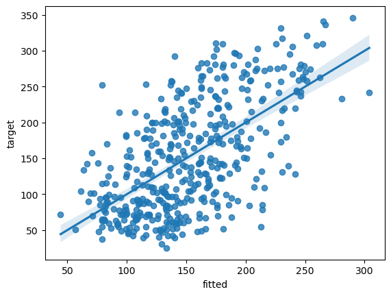
fit_lin = pd.DataFrame({'fitted':y_pred.squeeze(1).detach().numpy()})
fit_lin['target'] = df['target']

# plot model fits
fit_plot = sns.regplot(data=fit_lin, x="fitted", y="target")