4. Activation Functions

So far, we have looked at examples where the output is a weighted sum of the inputs. Generally, you’d use classical regression software in that case rather than torch, since the classical software provies greater speed and interpretability for linear regression. The benefit of deep learning is the ability to estimate nonlinear functions, which are generally beyond the scope of linear regression.

Nonlinearity is introduced to deep learning by using activation functions, which are simple, nonlinear functions that introduce complexity into the model. In this chapter, we will look at three of the most common activation functions: rectified linear units (ReLU), Sigmoid, and tanh. Let’s use the ReLU activation function as a specific example to understand how they work in a deep learning model.

4.1. ReLU Activation Function

Activation functions get their name from the Restricted Linear Unit (ReLU) activation function. It defines a threshold for its input and sets the output to zero if the input is below the threshold. Otherwise, the input is the same as the output. So, you could say that the output is active above the threshold and inactive below the threshold. Here is what the ReLU function looks like as it maps its input to its output:

The power of the ReLU activation function is that it introduces conditional statements like “if… then…” into the model. This allows the model to have different behavior depending on its inputs, rather than always giving the same weight to the same column of inputs. In order to make use of the complex conditionality, ReLU activation functions are typically put between linear layers. Here is an example that makes the linear regression model for diabetes progression into a nonlinear dep learning model:

# define the torch model
class NonlinearRegressionModel(torch.nn.Module):
    def __init__(self, input_dim, hidden_dim, output_dim=1):
        super(NonlinearRegressionModel, self).__init__()
        self.linear_1 = torch.nn.Linear(input_dim, hidden_dim)
        self.linear_2 = torch.nn.Linear(hidden_dim, output_dim)
        self.relu = torch.nn.ReLU(hidden_dim)


    def forward(self, x):
        result = self.linear_1(x)
        result = self.relu(result)
        result = self.linear_2(result)
        return result

Note that the model now has multipl linear layers with that operate on different dimensions and with a ReLU layer between them. We can now create an instance of the nonlinear model and train it:

# instantiate the model
my_nonlin = NonlinearRegressionModel(input_dim=2, hidden_dim=5)

# define the loss function and the optimizer
criterion = torch.nn.MSELoss()
optimizer = torch.optim.Adam(my_nonlin.parameters(), lr=1)

# convert the data to tensors
x_data = torch.tensor(df[['bmi', 's6']].values, dtype=torch.float32)
y_data = torch.tensor(df['target'].values, dtype=torch.float32).unsqueeze(-1)

# train the model by repeatedly making small steps toward the solution
for epoch in range(40000):
    # Forward pass
    y_pred = my_nonlin(x_data)
    
    # Compute and print loss
    loss = criterion(y_pred, y_data)
    if epoch % 1000 == 0:
        print(f'Epoch: {epoch} | Loss: {loss.item()}')
    
    # Zero gradients, perform a backward pass, and update the parameters.
    optimizer.zero_grad()
    loss.backward()
    optimizer.step()

Epoch: 0 | Loss: 29134.857421875

Epoch: 1000 | Loss: 3723.62890625

Epoch: 2000 | Loss: 3723.62890625

Epoch: 3000 | Loss: 3723.62890625

Epoch: 4000 | Loss: 3723.62841796875

Epoch: 5000 | Loss: 3723.62890625

Epoch: 6000 | Loss: 3723.628662109375

Epoch: 7000 | Loss: 3723.62890625

Epoch: 8000 | Loss: 3629.808349609375

Epoch: 9000 | Loss: 3631.943115234375

Epoch: 10000 | Loss: 3630.031982421875

Epoch: 11000 | Loss: 3629.775634765625

Epoch: 12000 | Loss: 3625.42822265625

Epoch: 13000 | Loss: 3625.53466796875

Epoch: 14000 | Loss: 3623.890625

Epoch: 15000 | Loss: 3624.219970703125

Epoch: 16000 | Loss: 3623.57568359375

Epoch: 17000 | Loss: 3625.212158203125

Epoch: 18000 | Loss: 3623.34521484375

Epoch: 19000 | Loss: 3623.49951171875

Epoch: 20000 | Loss: 3623.993896484375

Epoch: 21000 | Loss: 3623.3232421875

Epoch: 22000 | Loss: 3625.195068359375

Epoch: 23000 | Loss: 3622.60888671875

Epoch: 24000 | Loss: 3620.525390625

Epoch: 25000 | Loss: 3620.5341796875

Epoch: 26000 | Loss: 3620.423828125

Epoch: 27000 | Loss: 3620.857666015625

Epoch: 28000 | Loss: 3620.439697265625

Epoch: 29000 | Loss: 3622.558349609375

Epoch: 30000 | Loss: 3620.7119140625

Epoch: 31000 | Loss: 3620.645751953125

Epoch: 32000 | Loss: 3620.683349609375

Epoch: 33000 | Loss: 3620.650146484375

Epoch: 34000 | Loss: 3621.42822265625

Epoch: 35000 | Loss: 3620.89599609375

Epoch: 36000 | Loss: 3620.390380859375

Epoch: 37000 | Loss: 3621.003662109375

Epoch: 38000 | Loss: 3621.7138671875

Epoch: 39000 | Loss: 3620.70703125

The training loss seems stable after about 30000 iterations.

# print out the model parameters:
for param in my_nonlin.parameters():
    print(param)

Parameter containing:
tensor([[ -0.2555,  -0.5684],
        [ 80.6649,  32.7858],
        [ -5.8280,  -6.3134],
        [ 30.3064, -49.6007],
        [ 55.9338, 107.0210]], requires_grad=True)
Parameter containing:
tensor([-0.4508,  6.2032, -5.5858,  4.6875,  0.1389], requires_grad=True)
Parameter containing:
tensor([[-0.1531,  7.7079,  5.5726,  3.4063,  3.9982]], requires_grad=True)
Parameter containing:
tensor([76.4415], requires_grad=True)

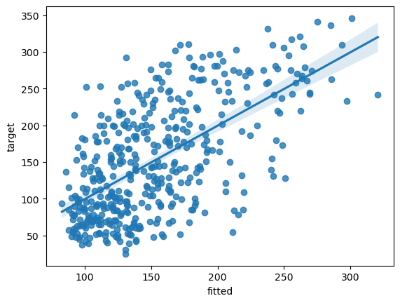
fit_nonlin = pd.DataFrame({'fitted':y_pred.squeeze(1).detach().numpy()})
fit_nonlin['target'] = df['target']

# plot model fits
fit_plot = sns.regplot(data=fit_nonlin, x="fitted", y="target")