1. Getting Started#
Learning Objectives
After this lesson, you should be able to:
Run code in a Python console (in JupyterLab)
Create variables
Call functions
Save and run code in a Jupyter notebook
Save, run, and import code in a module
Get or set Python’s working directory
Identify the format of a data file
Read a data set with Polars and inspect its contents
1.1. Why Python?#
Why should you use a programming language?
Code you write is reproducible: you can share it with someone else, and if they run it with the same inputs, they’ll get the same results. By writing code, you create an unambiguous record of every step taken in your analysis. This is one of the major advantages of programming languages over point-and-click software like Tableau or Microsoft Excel.
Another advantage of writing code is that it’s often reusable. This means you can:
Automate repetitive tasks within an analysis
Recycle code from one analysis into another
Package useful code for distribution to your colleagues or the general public
Python is a general-purpose programming language used in wide range of disciplines and industries. Its generality and popularity make knowing Python a valuable skill. Compared to other programming languages, some of Python’s particular strengths are its:
Easy-to-read syntax
Interactive interpreter and debugger
Idioms and culture that encourage explicit, straightforward code
Over 635,000 community-developed packages: reusable bundles of code, often accompanied by documentation, examples, or data sets
Flexible support for many different programming abstractions and paradigms
The main way you’ll interact with Python is by writing Python code or expressions. We’ll explain more soon, but first we need to install some packages that are critical for data science.
Note
The term “Python” can mean the Python language (the code) or the Python interpreter (the software which runs the code). Most of the time, the meaning is clear from the context, but we’ll be explicit in cases where the distinction is important.
1.1.1. Packages for Data Science#
Important
We recommend using Pixi to install and manage Python and Python packages.
Parts of this workshop require that you have Pixi installed on your computer and are familiar with how to use it. If you need a refresher, see DataLab’s Installing Software with Pixi workshop reader.
Python is general-purpose programming language, so data structures and functions specialized for research computing are not built-in. Instead, the community provides these through packages. Nevertheless, and to the community’s credit, Python is a leading language for research computing and data science. This section introduces some of the fundamental packages for research computing.
NumPy provides \(n\)-dimensional arrays (such as vectors and matrices) and a broad collection of mathematical functions. NumPy is the primary way to do linear algebra efficiently in Python. Many other packages depend on or are compatible with NumPy.
For data science, data frames, which represent tables of data, are another fundamental data structure. Several competing packages provide data frames and related functions:
Pandas is the oldest and most widely-used data frame package. It provides a broad set of features but also has many quirks. Pandas is generally less efficient than other packages in terms of compute time and memory usage.
Polars is specifically designed to be efficient, prevent bugs, and present a consistent programming interface. Polars is what we currently recommend for most people.
DuckDB treats data frames as tables in a database. This makes DuckDB extremely efficient and also means all operations on DuckDB data frames must be written in Structured Query Language (SQL) rather than Python. If you’re comfortable with SQL or need to work with big data (hundreds of gigabytes or more), DuckDB is a good choice.
Ibis provides data frames that can use any of the other packages under-the-hood. Ibis uses DuckDB by default, so it has similar efficiency but a Python programming interface (SQL is also supported).
We’ll use Polars, because it’s substantially more efficient than Pandas and provides early warnings for certain kinds of common mistakes.
Other notable packages for research computing in Python:
Jupyter provides interactive notebooks and IPython, a more convenient command-line prompt for Python.
SciPy provides even more mathematical functions, to supplement NumPy.
Matplotlib provides a rich collection of visualization functions and is the foundation for many data visualization packages.
statsmodels provides functions to fit statistical models (where the focus is inference and interpretability).
scikit-learn provides functions to fit machine learning models (where the focus is prediction). The package’s excellent documentation also provides a light but practical introduction to the models.
This is by no means an exhaustive list. You’re likely to encounter many more packages as you learn and use Python.
Important
To follow along with this chapter and the next, you’ll need an environment with Python, Jupyter, NumPy, and Polars.
You can use Pixi to create a project directory called python_basics with a
suitable environment. Open a terminal (such as Terminal or Git Bash) and run:
pixi init python_basics
cd python_basics
pixi add python jupyter numpy polars plotnine
After creating the environment, to launch JupyterLab in the enviroment, run:
pixi run jupyter lab
1.2. The JupyterLab Interface#
There are many different ways to edit and run Python code, but we’ll use JupyterLab. JupyterLab is an integrated development environment (IDE), which means it’s a comprehensive program for writing, editing, searching, and running code. You can do all of these things without JupyterLab, but JupyterLab makes the process easier.
The first time you open JupyterLab, you’ll see a window that looks like this:
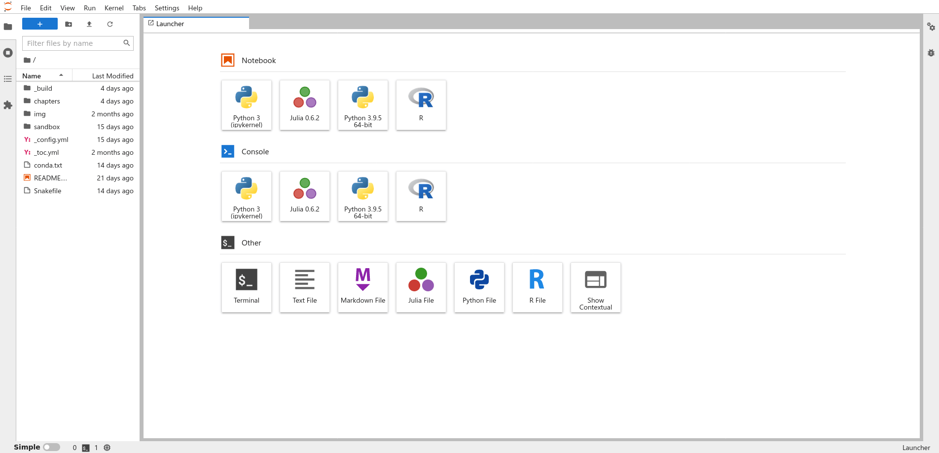
Fig. 1.1 The JupyterLab startup screen.#
Don’t worry if the text in the panes isn’t exactly the same on your computer; it depends on your operating system and version of JupyterLab.
Start by opening up a Python console. In JupyterLab, look for the “Python 3” button in the “Console” section of the pane on the right. If there are multiple Python 3 buttons, click on the one that mentions “IPython” or “ipykernel”:
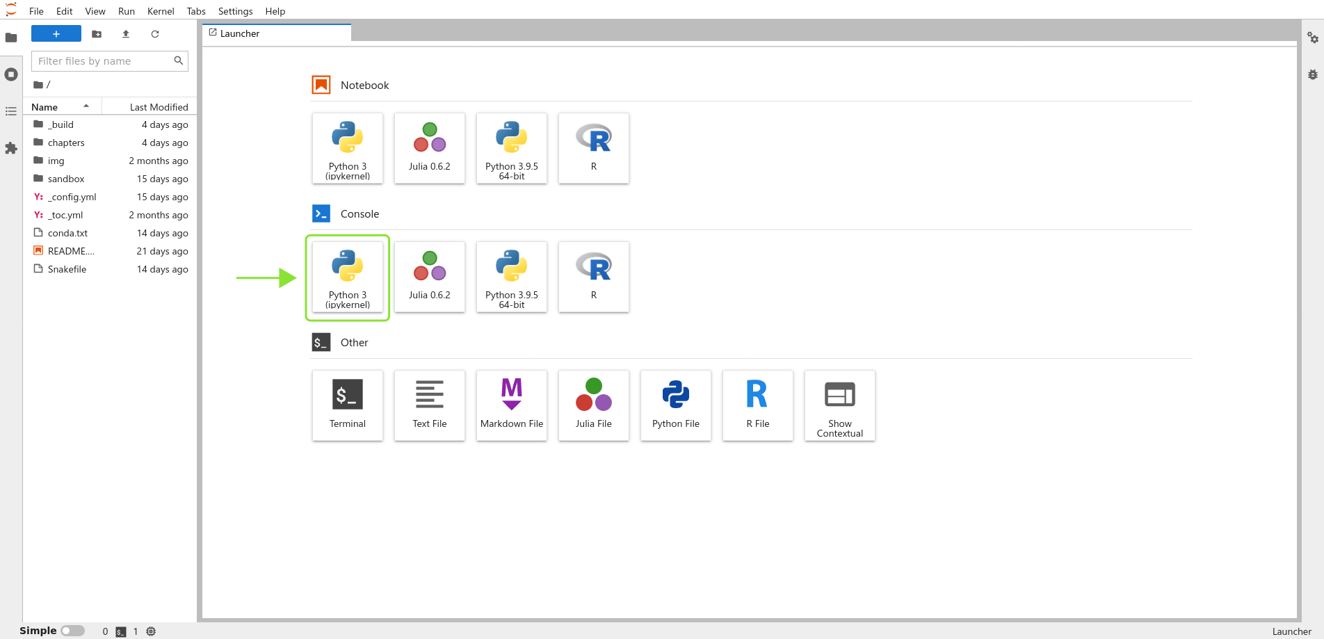
Fig. 1.2 The JupyterLab startup screen with the console button highlighted.#
The console is a interactive, text-based interface to Python. If you enter a Python expression in the console, Python will compute and display the result. After you open the console, your window should look like this:
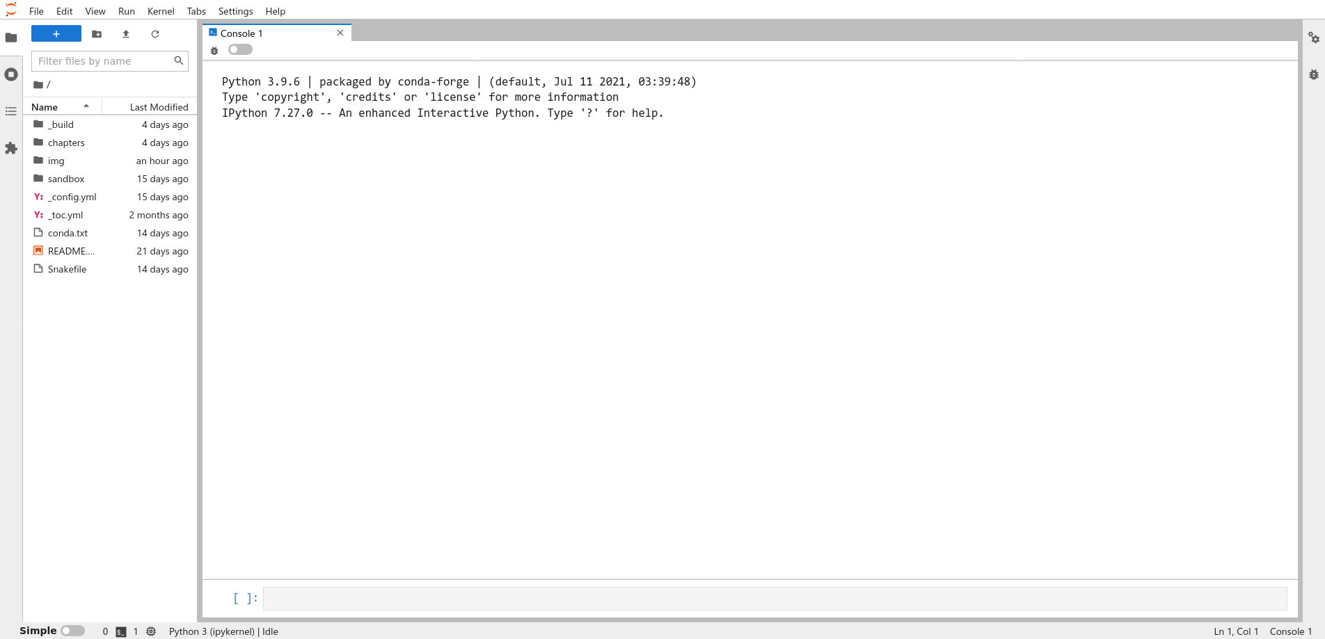
Fig. 1.3 A Python console running in JupyterLab.#
At the bottom of the console, the text box beginning with [ ]: is called the
prompt. The prompt is where you’ll type Python expressions. Ask Python to
compute the sum \(2 + 2\) by typing the code 2 + 2 in the prompt and then
pressing Shift-Enter. Your code and the result from Python should look like
this:
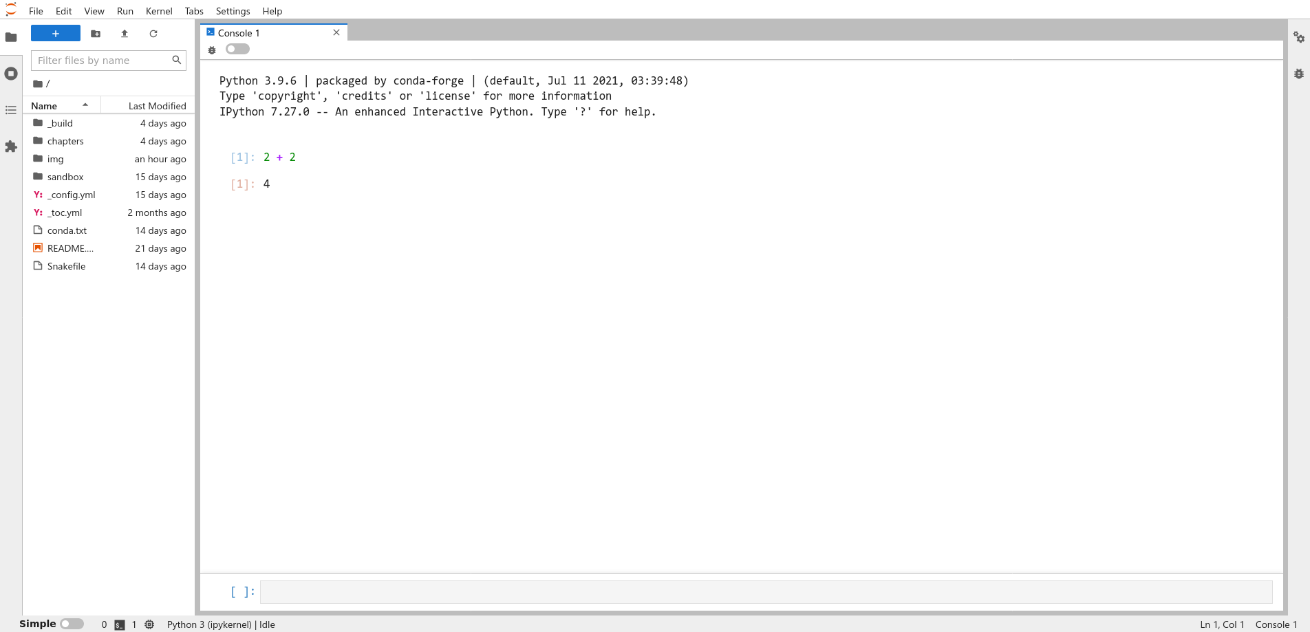
Fig. 1.4 A Python console running in JupyterLab, showing the sum of two numbers.#
The Python console displays your code and the result on separate lines. Both
begin with the tag [1] to indicate that they are the first expression and
result. Python will increment the tag each time you run an expression. The tag
numbers will restart from 1 each time you open a new Python console.
Now try typing the code 3 - 1 in the prompt and pressing Shift-Enter:
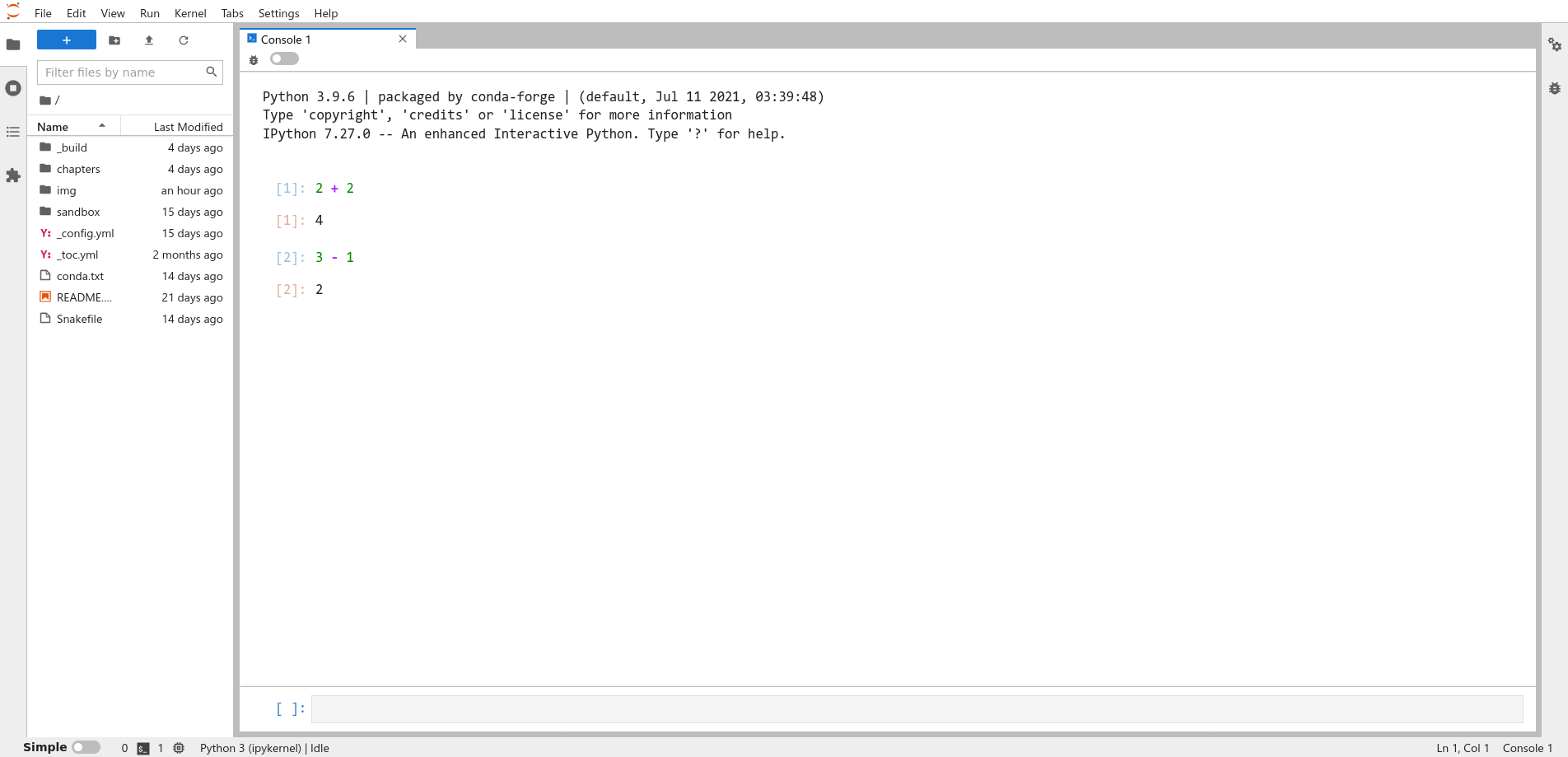
Fig. 1.5 A Python console running in JupyterLab, showing the difference of two numbers.#
The tag on the code and result is [2], and once again the result is displayed
after the tag.
1.3. Python Basics#
Try out some other arithmetic in the Python console. Besides + for addition,
the other arithmetic operators are:
-for subtraction*for multiplication/for division%for remainder division (modulo)**for exponentiation
You can combine these and use parentheses ( ) to make more complicated
expressions, just as you would when writing a mathematical expression. When
Python computes a result, it follows the standard order of operations:
parentheses, exponentiation, multiplication, division, addition, and finally
subtraction.
For example, to compute the area of a triangle, \(\frac{1}{2} (\textrm{base})(\textrm{height})\), with base 3 and height 4, you can write:
3 * 4 / 2
6.0
You can write Python expressions with any number of spaces (including none) around the operators and Python will still compute the result. Later on, you’ll learn about other kinds of expressions where the spacing does matter.
Tip
Use spaces!
As with writing text, putting spaces in your code makes it easier for you and others to read, so it’s good to make it a habit. Put a single space on each side of most operators, after commas, and after keywords.
1.3.1. Variables#
Python and most other programming languages allow you to create named values
called variables. You can create a variable with the assignment operator
= by writing a name on the left-hand side and a value or expression on the
right hand side. For example, to save the estimated area of the triangle in a
variable called area, you can write:
area = 3 * 4 / 2
In Python, variable names can consist of any combination of letters and
underscores (_). Names can also include numbers, but can’t start with a
number. Spaces, dots (.), and other symbols are not allowed in variable
names. So geese, top50dogs and nine_lives are valid variable names, but
goose teeth, tropical.fish and 9_lives are not.
Note
The official Python style guide, PEP 8, recommends against using capital letters in variable names even though Python allows it. Capital letters are conventionally used for other kinds of names. Following the recommendation will make your code easier for other Python programmers to understand.
The main reason to use variables is to temporarily save results from
expressions so that you can use them in other expressions. For instance, now
you can use the area variable anywhere you want the area of the triangle.
Notice that when you assign a result to a variable, Python doesn’t automatically display that result. If you want to see the result as well, you have to enter the variable’s name as a separate expression:
area
6.0
Another reason to use variables is to make an expression clearer and more
general. For instance, you might want to compute the area of several triangles
with different bases and heights. Then the expression 3 * 4 / 2 is too
specific. Instead, you can create variables base and height, then rewrite
the expression as base * height / 2. This makes the expression easier to
understand, because the reader does not have to intuit that 3 and 4 are the
base and height in the formula. Here’s the new code to compute and display the
area of a triangle with base 3 and height 4:
base = 3
height = 4
area = base * height / 2
area
6.0
Now if you want to compute the area for a different triangle, all you have to
do is change base and height and run the code again (Python will not update
area until you do this). Writing code that’s general enough to reuse across
multiple problems can be a big time-saver in the long run. Later on, you’ll see
ways to make this code even easier to reuse.
Tip
Try to choose descriptive variable names, so that you and your collaborators can understand the meaning and purpose of each variable when reading the code.
1.3.2. Strings#
Python treats anything inside single or double quotes as literal text rather than as an expression to evaluate. In programming jargon, a piece of literal text is called a string. You can use whichever kind of quotes you prefer, but the quote at the beginning of the string must match the quote at the end.
'Hi'
'Hi'
"Hello!"
'Hello!'
Numbers and strings are not the same thing, so for example Python considers 1
different from "1". You can use the number 1 in mathematical expressions,
but not the string "1".
1.3.3. Comparisons#
Besides arithmetic, you an also use Python to compare values. Programming tasks often involve comparing values. Use comparison operators to do so:
Operator |
Meaning |
|---|---|
|
less than |
|
greater than |
|
less than or equal to |
|
greater than or equal to |
|
equal to |
|
not equal to |
Notice that the “equal to” operator is two equal signs. This is to distinguish
it from the assignment = operator.
Here are a few examples:
1.5 < 3
True
"a" > "b"
False
3 == 3.14
False
"hi" == "hi"
True
When you make a comparison, Python returns a Boolean value. There are only
two possible Boolean values: True and False. Booleans are commonly used for
expressions with yes-or-no responses.
Boolean values are values, so you can use them in other computations. For example:
True
True
True == False
False
Tip
Python supports chained comparisons. For example, if you want to test whether
x is between 1 and 2, you can write:
1 < x < 2
This is syntactic sugar (a shortcut) for a longer expression:
1 < x and x < 2
You can use any of the comparison operators in chained comparisons, and Python
will implicitly combine each comparison with and.
1.3.4. Calling Functions#
Python can do a lot more than just arithmetic. Most of Python’s features are provided through functions, pieces of reusable code. You can think of a function as a machine that takes some inputs and uses them to produce some output. In programming jargon, the inputs to a function are called arguments, the output is called the return value, and when you use a function, you’re calling the function.
To call a function, write its name followed by parentheses. Put any arguments
to the function inside the parentheses. For example, the function to round a
number to a specified decimal place is named round. So you can round the
number 8.153 to the nearest integer with this code:
round(8.153)
8
Many functions accept more than one argument. For instance, the round
function accepts two arguments: the number to round, and the number of decimal
places to keep. When you call a function with multiple arguments, separate the
arguments with commas. So to round 8.153 to 1 decimal place:
round(8.153, 1)
8.2
When you call a function, Python assigns the arguments to the function’s
parameters. Parameters are special variables that represent the inputs to a
function and only exist while that function runs. For example, the round
function has parameters number and ndigits. The next section,
Getting Help, explains how to look up the parameters for a function.
Some parameters have default arguments. A parameter is automatically
assigned its default argument whenever the parameter’s argument is not
specified explicitly. As a result, assigning arguments to these parameters is
optional. For instance, the ndigits parameter of round has a default
argument (round to the nearest integer), so it is okay to call round without
setting ndigits, as in round(8.153). In contrast, the numbers parameter
does not have a default argument. Getting Help explains how to look up
the default arguments for a function.
Python normally assigns arguments to parameters based on their position. The
first argument is assigned to the function’s first parameter, the second to the
second, and so on. So in the code above, 8.153 is assigned to number and
1 is assigned to ndigits.
You can make Python assign arguments to parameters by name with =, overriding
their positions. So some other ways you can write the call above are:
round(8.153, ndigits = 1)
8.2
round(number = 8.153, ndigits = 1)
8.2
round(ndigits = 1, number = 8.153)
8.2
All of these are equivalent. When you write code, choose whatever seems the clearest to you. Leaving parameter names out of calls saves typing, but including some or all of them can make the code easier to understand.
Parameters are not regular variables, and only exist while their associated function runs. You can’t set them before a call, nor can you access them after a call. So this code causes an error:
number = 4.755
round(ndigits = 2)
---------------------------------------------------------------------------
TypeError                                 Traceback (most recent call last)
Cell In[19], line 2
      1 number = 4.755
----> 2 round(ndigits = 2)

TypeError: round() missing required argument 'number' (pos 1)
In the error message, Python says that you forgot to assign an argument to the
parameter number. You can keep the variable number and correct the call by
making number an argument (for the parameter number):
round(number, ndigits = 2)
4.75
Note
It might be surprising that Python’s round function rounds 4.755 to 4.75
instead of 4.76, but it’s not a bug. Most rounding functions are
slightly inaccurate because of how computers represent decimal numbers.
NumPy provides its own rounding function, np.round, which uses a different,
faster rounding algorithm and may give different results.
Or, written more explicitly:
round(number = number, ndigits = 2)
4.75
The point is that variables and parameters are distinct, even if they happen to
have the same name. The variable number is not the same thing as the
parameter number.
1.3.5. Objects & Attributes#
Python represents data as objects. Numbers, strings, data structures, and functions are all examples of objects.
An attribute is an object attached to another object. An attribute usually
contains metadata about the object to which it is attached. You can access
attributes by typing a . after an object.
When an attribute is a function, it’s called a method. For example, all
strings have a capitalize method. Here’s the code to capitalize a string:
"snakes everywhere!".capitalize()
'Snakes everywhere!'
The built-in dir function lists all of the attributes attached to
an object. Here are the attributes for a string:
dir("hi")
['__add__',
 '__class__',
 '__contains__',
 '__delattr__',
 '__dir__',
 '__doc__',
 '__eq__',
 '__format__',
 '__ge__',
 '__getattribute__',
 '__getitem__',
 '__getnewargs__',
 '__getstate__',
 '__gt__',
 '__hash__',
 '__init__',
 '__init_subclass__',
 '__iter__',
 '__le__',
 '__len__',
 '__lt__',
 '__mod__',
 '__mul__',
 '__ne__',
 '__new__',
 '__reduce__',
 '__reduce_ex__',
 '__repr__',
 '__rmod__',
 '__rmul__',
 '__setattr__',
 '__sizeof__',
 '__str__',
 '__subclasshook__',
 'capitalize',
 'casefold',
 'center',
 'count',
 'encode',
 'endswith',
 'expandtabs',
 'find',
 'format',
 'format_map',
 'index',
 'isalnum',
 'isalpha',
 'isascii',
 'isdecimal',
 'isdigit',
 'isidentifier',
 'islower',
 'isnumeric',
 'isprintable',
 'isspace',
 'istitle',
 'isupper',
 'join',
 'ljust',
 'lower',
 'lstrip',
 'maketrans',
 'partition',
 'removeprefix',
 'removesuffix',
 'replace',
 'rfind',
 'rindex',
 'rjust',
 'rpartition',
 'rsplit',
 'rstrip',
 'split',
 'splitlines',
 'startswith',
 'strip',
 'swapcase',
 'title',
 'translate',
 'upper',
 'zfill']
Caution
Attributes that begin with two underscores __ are used by Python internally
and are usually not intended to be accessed directly.
1.4. Getting Help#
Learning and using a language is hard, so it’s important to know how to get
help. The first place to look for help is Python’s built-in documentation. In
the console, you can access the help pages with the help function.
There are help pages for all of Python’s built-in functions, usually with the
same name as the function itself. So the code to open the help page for the
round function is:
help(round)
Help on built-in function round in module builtins:

round(number, ndigits=None)
    Round a number to a given precision in decimal digits.

    The return value is an integer if ndigits is omitted or None.  Otherwise
    the return value has the same type as the number.  ndigits may be negative.
For functions, help pages usually include a brief description and a list of
parameters and default arguments. For instance, the help page for round shows
that there are two parameters number and ndigits. It also says that
ndigits=None, meaning the default argument for ndigits is the special
None value (you’ll learn more about None in Special Values).
There are also help pages for other topics, such as built-in operators and modules (you’ll learn about modules in Saving & Loading Code). To look up the help page for an operator, put the operator’s name in single or double quotes. For example, this code opens the help page for the arithmetic operators:
help("+")
Operator precedence
*******************

The following table summarizes the operator precedence in Python, from
highest precedence (most binding) to lowest precedence (least
binding).  Operators in the same box have the same precedence.  Unless
the syntax is explicitly given, operators are binary.  Operators in
the same box group left to right (except for exponentiation and
conditional expressions, which group from right to left).

Note that comparisons, membership tests, and identity tests, all have
the same precedence and have a left-to-right chaining feature as
described in the Comparisons section.

+-------------------------------------------------+---------------------------------------+
| Operator                                        | Description                           |
|=================================================|=======================================|
| "(expressions...)",  "[expressions...]", "{key: | Binding or parenthesized expression,  |
| value...}", "{expressions...}"                  | list display, dictionary display, set |
|                                                 | display                               |
+-------------------------------------------------+---------------------------------------+
| "x[index]", "x[index:index]",                   | Subscription, slicing, call,          |
| "x(arguments...)", "x.attribute"                | attribute reference                   |
+-------------------------------------------------+---------------------------------------+
| "await x"                                       | Await expression                      |
+-------------------------------------------------+---------------------------------------+
| "**"                                            | Exponentiation [5]                    |
+-------------------------------------------------+---------------------------------------+
| "+x", "-x", "~x"                                | Positive, negative, bitwise NOT       |
+-------------------------------------------------+---------------------------------------+
| "*", "@", "/", "//", "%"                        | Multiplication, matrix                |
|                                                 | multiplication, division, floor       |
|                                                 | division, remainder [6]               |
+-------------------------------------------------+---------------------------------------+
| "+", "-"                                        | Addition and subtraction              |
+-------------------------------------------------+---------------------------------------+
| "<<", ">>"                                      | Shifts                                |
+-------------------------------------------------+---------------------------------------+
| "&"                                             | Bitwise AND                           |
+-------------------------------------------------+---------------------------------------+
| "^"                                             | Bitwise XOR                           |
+-------------------------------------------------+---------------------------------------+
| "|"                                             | Bitwise OR                            |
+-------------------------------------------------+---------------------------------------+
| "in", "not in", "is", "is not", "<", "<=", ">", | Comparisons, including membership     |
| ">=", "!=", "=="                                | tests and identity tests              |
+-------------------------------------------------+---------------------------------------+
| "not x"                                         | Boolean NOT                           |
+-------------------------------------------------+---------------------------------------+
| "and"                                           | Boolean AND                           |
+-------------------------------------------------+---------------------------------------+
| "or"                                            | Boolean OR                            |
+-------------------------------------------------+---------------------------------------+
| "if" – "else"                                   | Conditional expression                |
+-------------------------------------------------+---------------------------------------+
| "lambda"                                        | Lambda expression                     |
+-------------------------------------------------+---------------------------------------+
| ":="                                            | Assignment expression                 |
+-------------------------------------------------+---------------------------------------+

-[ Footnotes ]-

[1] While "abs(x%y) < abs(y)" is true mathematically, for floats it
    may not be true numerically due to roundoff.  For example, and
    assuming a platform on which a Python float is an IEEE 754 double-
    precision number, in order that "-1e-100 % 1e100" have the same
    sign as "1e100", the computed result is "-1e-100 + 1e100", which
    is numerically exactly equal to "1e100".  The function
    "math.fmod()" returns a result whose sign matches the sign of the
    first argument instead, and so returns "-1e-100" in this case.
    Which approach is more appropriate depends on the application.

[2] If x is very close to an exact integer multiple of y, it’s
    possible for "x//y" to be one larger than "(x-x%y)//y" due to
    rounding.  In such cases, Python returns the latter result, in
    order to preserve that "divmod(x,y)[0] * y + x % y" be very close
    to "x".

[3] The Unicode standard distinguishes between *code points* (e.g.
    U+0041) and *abstract characters* (e.g. “LATIN CAPITAL LETTER A”).
    While most abstract characters in Unicode are only represented
    using one code point, there is a number of abstract characters
    that can in addition be represented using a sequence of more than
    one code point.  For example, the abstract character “LATIN
    CAPITAL LETTER C WITH CEDILLA” can be represented as a single
    *precomposed character* at code position U+00C7, or as a sequence
    of a *base character* at code position U+0043 (LATIN CAPITAL
    LETTER C), followed by a *combining character* at code position
    U+0327 (COMBINING CEDILLA).

    The comparison operators on strings compare at the level of
    Unicode code points. This may be counter-intuitive to humans.  For
    example, ""\u00C7" == "\u0043\u0327"" is "False", even though both
    strings represent the same abstract character “LATIN CAPITAL
    LETTER C WITH CEDILLA”.

    To compare strings at the level of abstract characters (that is,
    in a way intuitive to humans), use "unicodedata.normalize()".

[4] Due to automatic garbage-collection, free lists, and the dynamic
    nature of descriptors, you may notice seemingly unusual behaviour
    in certain uses of the "is" operator, like those involving
    comparisons between instance methods, or constants.  Check their
    documentation for more info.

[5] The power operator "**" binds less tightly than an arithmetic or
    bitwise unary operator on its right, that is, "2**-1" is "0.5".

[6] The "%" operator is also used for string formatting; the same
    precedence applies.

Related help topics: lambda, or, and, not, in, is, BOOLEAN, COMPARISON,
BITWISE, SHIFTING, BINARY, FORMATTING, POWER, UNARY, ATTRIBUTES,
SUBSCRIPTS, SLICINGS, CALLS, TUPLES, LISTS, DICTIONARIES
It’s always okay to put quotes around the name of the page when you use help,
but they’re only required if the name contains non-alphabetic characters. So
help(abs), help('abs'), and help("abs") all open the documentation for
abs, the absolute value function.
You can also browse the Python documentation online. This is a good way to explore the many different functions and data structures built into Python.
Important
If you do use the online documentation, make sure to use the documentation for the same version of Python as the one you have. Python displays the version each time you open a new console, and the online documentation shows the version in the upper left corner.
Sometimes you might not know the name of the help page you want to look up. In that case it’s best to use an online search engine. When you search for help with Python online, include “Python” as a search term.
1.4.1. When Something Goes Wrong#
As a programmer, sooner or later you’ll run some code and get an error message or result you didn’t expect. Don’t panic! Even experienced programmers make mistakes regularly, so learning how to diagnose and fix problems is vital.
Try going through these steps:
If Python printed a warning or error message, read it! If you’re not sure what the message means, try searching for it online.
Check your code for typographical errors, including incorrect capitalization, whitespace, and missing or extra commas, quotes, and parentheses.
Test your code one line at a time, starting from the beginning. After each line that assigns a variable, check that the value of the variable is what you expect. Try to determine the exact line where the problem originates (which may differ from the line that emits an error!).
If none of these steps help, try asking online. Stack Overflow is a popular question and answer website for programmers. Before posting, make sure to read about how to ask a good question.
1.5. Saving & Loading Code#
Tip
When you start a new project, it’s a good idea to create a specific directory for all of the project’s files. If you’re using Python, you should also store your Python code in that directory. As you work, periodically save your code.
Most of the time, you won’t just write code directly into the Python console. Reproducibility and reusability are important benefits of Python over point-and-click software, and in order to realize these, you have to save your code to your computer’s hard drive.
The most common way to save Python code is as a Python module (or script)
with the extension .py (see Reading Files for more about extensions).
Editing a module is similar to editing any other text document. You can write,
delete, copy, cut, and paste code.
You can create a new Python module in JupyterLab with this menu option:
File -> New -> Python File
Every line in a Python module must be valid Python code. Anything else you want to write in the module (notes, documentation, etc.) must be placed in a comment.
Arrange your code in the order of the steps to solve the problem, even if you write some parts before others. Comment out or delete any lines of code that you try but ultimately decide you don’t need. Make sure to save the file periodically so that you don’t lose your work. Following these guidelines will help you stay organized and make it easier to share your code with others later.
1.5.1. Importing Modules#
You can import a module with the import command. Python will run the
module’s code so that you can use any functions or data structures it defines.
There are many modules built into Python that provide extra functionality. In
addition, every package consists of one or more modules.
Tip
The best way to learn about the modules in a package is to read the package’s documentation.
Most packages have a main module with the same name as the package. So the
NumPy package provides a module called numpy, and the Polars package provides
a module called polars. Make sure you have NumPy installed, then try loading
the numpy module:
import numpy
A handful of modules print out a message when loaded, but the vast majority do
not. Thus you can assume the import command was successful if nothing is
printed. If something goes wrong while loading a module, Python will print out
an error message explaining the problem.
Once a module is imported, you can access its functions by typing the name of
the module, a dot ., and then the name of the function. For instance, to use
the round function provided by NumPy:
numpy.round(3.3)
np.float64(3.0)
Important
NumPy’s np.round is an entirely different function than Python’s built-in
round function, even though they do the same thing. NumPy’s math functions
are generally faster, more precise, and more convenient than Python’s built-in
math functions.
Typing the full name of a module is inconvenient, so the import command
allows you to define an alias when you import a module. For popular packages,
there’s usually a conventional alias for the main module. The conventional
alias for numpy is np. Using the conventional alias is a good habit,
because it makes it easier for other people to understand your code. Use the
as keyword to set an alias when you import a module:
import numpy as np
Now you can call NumPy functions by typing np instead of numpy:
np.round(3.4)
np.float64(3.0)
Note
You can also use the import command to import code from one of your modules
into another. The module you want to import must be saved somewhere Python can
find it. One way to do this is to put the module you want to import in the
same directory as the module that will import it.
1.5.2. Jupyter Notebooks#
For data science tasks, it is also common to use a Jupyter notebook with
extension .ipynb to store code. In addition to Python code, Jupyter notebooks
have full support for formatted text, images, and code from other programming
languages such as Julia and R. The tradeoff is that Jupyter notebooks can only
be viewed in a web browser.
Note
“Jupyter” is short for “Julia, Python, Text, and R.”
Jupyter notebooks are more convenient than Python scripts for interactive work such as data analysis and learning or experimenting with the language. On the other hand, Python scripts are more appropriate for long-running code that does not require user interaction (such as web scrapers or scientific simulations) and for developing packages and software. The remainder of this reader assumes you’re using a Jupyter notebook rather than the Python console or a Python script, unless otherwise noted.
You can create a new Jupyter notebook in JupyterLab with this menu option:
File -> New -> Notebook
JupyterLab will prompt you to select a kernel for the notebook. The kernel is the software used to run code in the notebook. For a notebook that will contain Python code, you should choose a Python kernel.
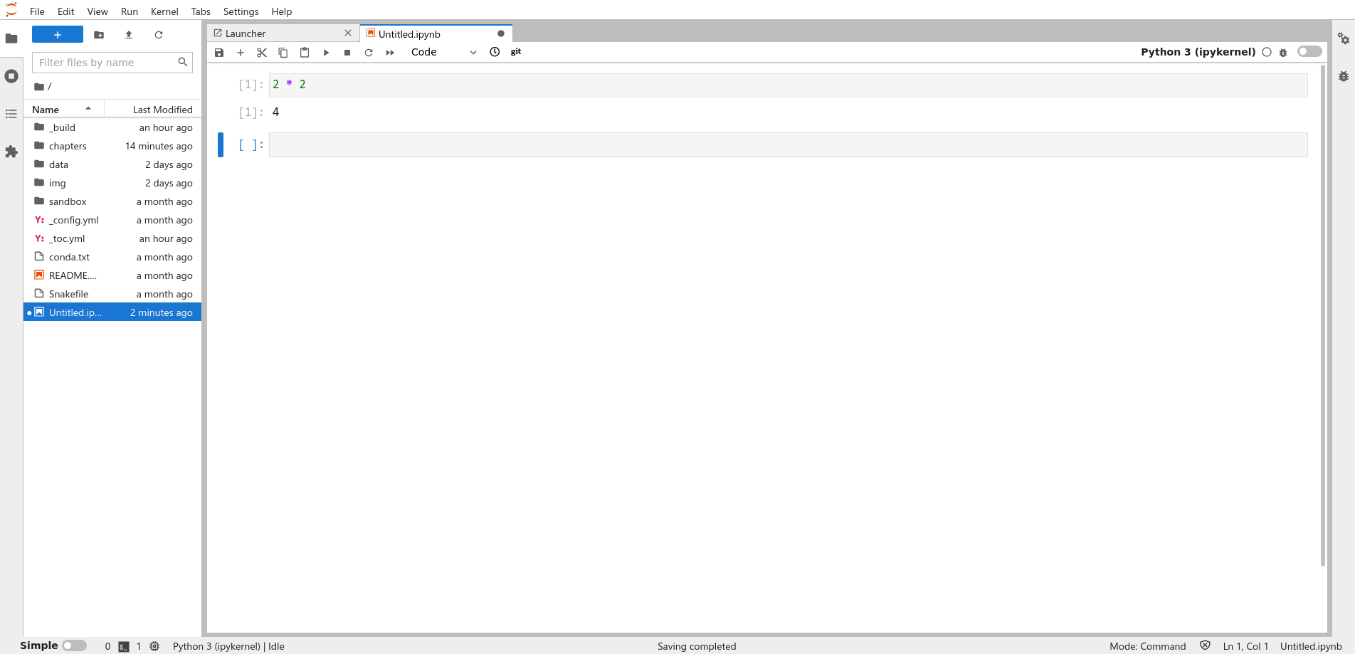
After you select the kernel, you’ll see a pane like this:

Jupyter notebooks are subdivided into cells. You can create as many cells as you like, but each cell can only contain one kind of content, usually code or text.
New cells are code cells by default. You can run a code cell by clicking on the
cell and pressing Shift-Enter. The notebook will display the result and
create a new empty code cell below the result:
You can convert a code cell to a text cell by clicking on the cell and selecting the “Markdown” option from the cell type dropdown menu:
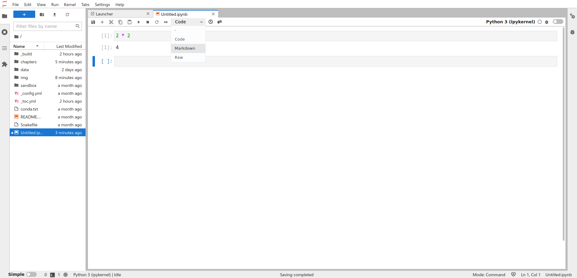
Markdown is a simple language you can use to add formatting to your text. For
example, surrounding a word with asterisks, as in Let *sleeping* dogs lie,
makes the surrounded word italic. You can find a short, interactive tutorial
about Markdown here. If you “run” a text cell by pressing
Shift-Enter, the notebook will display the text with any formatting you
added.
1.6. File Systems#
This section is a review of how files on a computer work. You’ll need to understand this in order to read a data set from a file, and it’s also important for finding your saved notebooks and modules later.
Your computer’s file system consists of files (chunks of data) and directories (or “folders”) to organize those files. For instance, the file system on a computer shared by Ada and Charles, two pioneers of computing, might look like this:
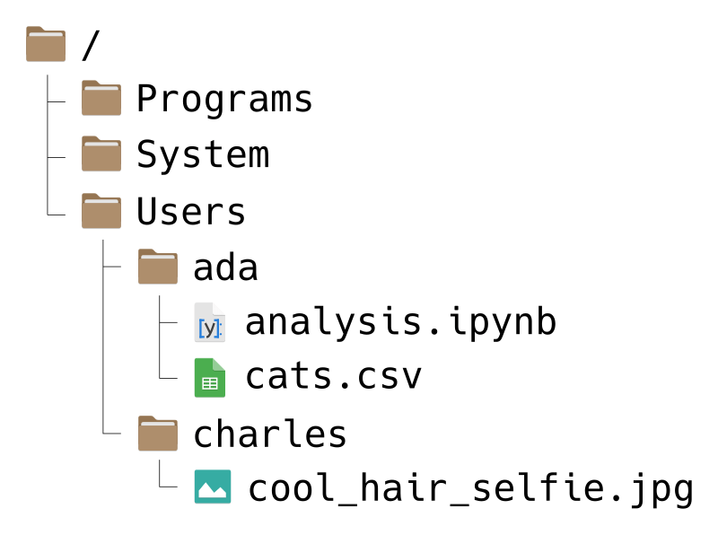
Don’t worry if your file system looks a bit different from the picture.
File systems have a tree-like structure, with a top-level directory called the
root directory. On Ada and Charles’ computer, the root is called /, which
is also what it’s called on all macOS and Linux computers. On Windows, the root
is usually called C:/, but sometimes other letters, like D:/, are also used
depending on the computer’s hardware.
A path is a list of directories that leads to a specific file or directory
on a file system (imagine giving directions to someone as they walk through the
file system). Use forward slashes / to separate the directories in a path,
rather than commas or spaces. The root directory includes a forward slash as
part of its name, and doesn’t need an extra one.
For example, suppose Ada wants to write a path to the file cats.csv. She can
write the path like this:
/Users/ada/cats.csv
You can read this path from left-to-right as, “Starting from the root
directory, go to the Users directory, then from there go to the ada
directory, and from there go to the file cats.csv.” Alternatively, you can
read the path from right-to-left as, “The file cats.csv inside of the ada
directory, which is inside of the Users directory, which is in the root
directory.”
As another example, suppose Charles wants a path to the Programs directory.
He can write:
/Programs/
The / at the end of this path is reminder that Programs is a directory, not
a file. Charles could also write the path like this:
/Programs
This is still correct, but it’s not as obvious that Programs is a directory.
In other words, when a path leads to a directory, including a trailing
slash is optional, but makes the meaning of the path clearer. Paths that lead
to files never have a trailing slash.
Warning
On Windows computers, the components of a path are usually separated with
backslashes \ instead of forward slashes /.
Regardless of the operating system, most Python functions accept and understand paths separated with forward slashes as arguments. In other words, you can use paths separated with forward slashes in your Python code, even on Windows. This is especially convenient when you want to share code with other people, because they might use a different operating system than you.
On Windows, most Python functions return paths separated by backslashes. Be
careful of this if your code gets a path by calling a function and then edits
it (for example, by calling os.getcwd and then splitting the path into its
components). The separator will be a backslash on Windows, but a forward slash
on all other operating systems. Python’s built-in pathlib module provides
helper functions to edit paths that account for differences between operating
systems.
1.6.1. Absolute & Relative Paths#
A path that starts from the root directory, like all of the ones we’ve seen so far, is called an absolute path. The path is “absolute” because it unambiguously describes where a file or directory is located. The downside is that absolute paths usually don’t work well if you share your code.
For example, suppose Ada uses the path /Programs/ada/cats.csv to load the
cats.csv file in her code. If she shares her code with another pioneer of
computing, say Gladys, who also has a copy of cats.csv, it might
not work. Even though Gladys has the file, she might not have it in a directory
called ada, and might not even have a directory called ada on her computer.
Because Ada used an absolute path, her code works on her own computer, but
isn’t portable to others.
On the other hand, a relative path is one that doesn’t start from the root directory. The path is “relative” to an unspecified starting point, which usually depends on the context.
For instance, suppose Ada’s code is saved in the file analysis.ipynb, which
is in the same directory as cats.csv on her computer. Then instead of an
absolute path, she can use a relative path in her code:
cats.csv
The context is the location of analysis.ipynb, the file that contains the
code. In other words, the starting point on Ada’s computer is the ada
directory. On other computers, the starting point will be different, depending
on where the code is stored.
Now suppose Ada sends her corrected code in analysis.ipynb to Gladys, and
tells Gladys to put it in the same directory as cats.csv. Since the path
cats.csv is relative, the code will still work on Gladys’ computer, as long
as the two files are in the same directory. The name of that directory and its
location in the file system don’t matter, and don’t have to be the same as on
Ada’s computer. Gladys can put the files in a directory
/Users/gladys/from_ada/ and the path (and code) will still work.
Relative paths can include directories. For example, suppose that Charles wants
to write a relative path from the Users directory to a cool selfie he took.
Then he can write:
charles/cool_hair_selfie.jpg
You can read this path as, “Starting from wherever you are, go to the charles
directory, and from there go to the cool_hair_selfie.jpg file.” In other
words, the relative path depends on the context of the code or program that
uses it.
Tip
When you use paths in code, they should almost always be relative paths. This ensures that the code is portable to other computers, which is an important aspect of reproducibility. Another benefit is that relative paths tend to be shorter, making your code easier to read (and write).
When you write paths, there are three shortcuts you can use. These are most useful in relative paths, but also work in absolute paths:
.means the current directory...means the directory above the current directory.~means the home directory. Each user has their own home directory, whose location depends on the operating system and their username. Home directories are typically found insideC:/Users/on Windows,/Users/on macOS, and/home/on Linux.
As an example, suppose Ada wants to write a (relative) path from the ada
directory to Charles’ cool selfie. Using these shortcuts, she can write:
../charles/cool_hair_selfie.jpg
Read this as, “Starting from wherever you are, go up one directory, then go to
the charles directory, and then go to the cool_hair_selfie.jpg file.” Since
/Users/ada is Ada’s home directory, she could also write the path as:
~/../charles/cool_hair_selfie.jpg
This path has the same effect, but the meaning is slightly different. You can
read it as “Starting from your home directory, go up one directory, then go to
the charles directory, and then go to the cool_hair_selfie.jpg file.”
The .. and ~ shortcut are frequently used and worth remembering. The .
shortcut is included here in case you see it in someone else’s code. Since it
means the current directory, a path like ./cats.csv is identical to
cats.csv, and the latter is preferable for being simpler. There are a few
specific situations where . is necessary, but they fall outside the scope of
this text.
1.6.2. The Working Directory#
Absolute & Relative Paths explained that relative paths have a starting point that depends on the context where the path is used. The working directory is the starting point Python uses for relative paths. Think of the working directory as the directory Python is currently “at” or watching.
Python’s built-in os module provides functions to manipulate the working
directory. The function os.getcwd returns the absolute path for the current
working directory, as a string. It doesn’t require any arguments:
import os

os.getcwd()
'/home/nick/mill/datalab/teaching/python_basics'
On your computer, the output from os.getcwd will likely be different. This is
a very useful function for getting your bearings when you write relative paths.
If you write a relative path and it doesn’t work as expected, the first thing
to do is check the working directory.
The related os.chdir function changes the working directory. It takes one
argument: a path to the new working directory. Here’s an example:
os.chdir("..")

# Now check the working directory.
os.getcwd()
'/home/nick/mill/datalab/teaching'
Warning
Generally, you should avoid using calls to os.chdir in your Jupyter notebooks
and Python scripts. Calling os.chdir makes your code more difficult to
understand, and can always be avoided by using appropriate relative paths. If
you call os.chdir with an absolute path, it also makes your code less
portable to other computers. It’s fine to use os.chdir interactively (in the
Python console), but avoid making your saved code dependent on it.
Another function that’s useful for dealing with the working directory and file
system is os.listdir. The os.listdir function returns the names of all of
the files and directories inside of a directory. It accepts a path to a
directory as an argument, or assumes the working directory if you don’t pass a
path. For instance:
# List files and directories in /home/.
os.listdir("/home/")

# List files and directories in the working directory.
os.listdir()
['bml-model',
 'python_intensive_training',
 'python_basics',
 'intro_to_machine_learning',
 'install_guides',
 'workshop_index',
 'reproducible_research',
 '2022_python_bootcamp',
 'testing',
 'intro_to_the_command_line',
 'intermediate_python',
 'workshop_regression',
 'workshop_ocr_python',
 'dynamic_data_viz',
 'adventures_in_data_science',
 'data_viz.md',
 'template_python_workshop',
 'ollama',
 'intro_qgis',
 'ocr',
 'template_r_workshop',
 'data_viz_principles',
 'r_basics',
 'statistics_notes',
 'archive',
 'jupyterbook-notes.md',
 '2021_remote_computing',
 '2024_adventures_in_data_science',
 'cradle',
 'intermediate_r',
 'workshop_handouts',
 'intro_to_sql',
 'intro_to_remote_computing',
 'julia_basics']
As usual, since you have a different computer, you’re likely to see different
output if you run this code. If you call os.listdir with an invalid path or
an empty directory, Python raises a FileNotFoundError:
os.listdir("/this/path/is/fake/")
---------------------------------------------------------------------------
FileNotFoundError                         Traceback (most recent call last)
Cell In[35], line 1
----> 1 os.listdir("/this/path/is/fake/")

FileNotFoundError: [Errno 2] No such file or directory: '/this/path/is/fake/'
1.7. Reading Files#
The first step in most data analyses is loading a data set. The Polars package provides functions to read data sets saved in a variety of file formats. In order to know which function to use, you must first identify the file format.
Most of the time, you can guess the format of a file by looking at its
extension, the characters (usually three) after the last dot . in the
filename. For example, the extension .jpg or .jpeg indicates a JPEG image
file. Some operating systems hide extensions by default, but you can find
instructions to change this setting online by searching for “show file
extensions” and your operating system’s name. The extension is just part of the
file’s name, so it should be taken as a hint about the file’s format rather
than a guarantee.
The table below shows several formats that are frequently used to distribute data. Polars provides reader functions for many of these, but some can only be read with help from other packages or Python’s built-in modules.
Name |
Extension |
Function or Package |
Tabular? |
Text? |
|---|---|---|---|---|
Comma-separated Values |
|
|
Yes |
Yes |
Tab-separated Values |
|
|
Yes |
Yes |
Fixed-width File |
|
See this issue |
Yes |
Yes |
Microsoft Excel |
|
|
Yes |
No |
|
|
Yes |
No |
|
|
|
Yes |
No |
|
Extensible Markup Language |
|
parsel package |
No |
Yes |
JavaScript Object Notation |
|
|
No |
Yes |
Arbitrary File |
|
A tabular data set is one that’s structured as a table, with rows and columns. We’ll focus on tabular data sets for most of this reader, since they’re easier to get started with. Here’s an example of a tabular data set:
Fruit |
Quantity |
Price |
|---|---|---|
apple |
32 |
1.49 |
banana |
541 |
0.79 |
pear |
10 |
1.99 |
A text file is one that contains human-readable lines of text. You can check this by opening the file with a text editor such as Microsoft Notepad or macOS TextEdit. Many file formats use text in order to make the format easier to work with.
For instance, a comma-separated values (CSV) file records a tabular data using one line per row, with commas separating columns. If you store the table above in a CSV file and open the file in a text editor, here’s what you’ll see:
Fruit,Quantity,Price
apple,32,1.49
banana,541,0.79
pear,10,1.99
A binary file is one that’s not human-readable. You can’t just read off the data if you open a binary file in a text editor, but they have a number of other advantages. Compared to text files, binary files are often faster to read and take up less storage space (bytes).
1.7.1. Hello, Data!#
The California least tern is a endangered subspecies of seabird that nests along the coast of California and Mexico. The California Department of Fish and Wildlife (CDFW) monitors least tern nesting sites across the state to estimate breeding pairs, fledglings, and predator activity in each annual breeding season.

Fig. 1.6 A California least tern. Original photo by Mark Pavelka, U.S. Fish & Wildlife Service (CC BY 2.0).#
The CDFW publishes most of the data it collects to the California Open Data portal. The examples in this and subsequent chapters use a cleaned 2000-2023 version of the California least tern data.
Important
Click here to download the 2000-2023 California least tern data set.
If you haven’t already, we recommend you create a directory for this workshop.
In your workshop directory, create a data/ subdirectory. Download and save
the California least tern data set in the data/ subdirectory.
Documentation for 2000-2023 California Least Tern Data Set
Each row in the data set contains measurements from one year-site combination.
Column |
Description |
|---|---|
|
Year of the breeding season |
|
Site name |
|
Site name from 2013-2018 |
|
Site name from 1988-2001 |
|
Abbreviated site name |
|
Region of state: S.F. Bay, Central, or Southern (includes Ventura) |
|
Region of state: S.F. Bay, Central, Ventura, or Southern |
|
Climate events |
|
Reported minimum breeding pairs |
|
Reported maximum breeding pairs |
|
Reported minimum fledges |
|
Reported maximum fledges |
|
Total reported nests (maximum if a range was reported) |
|
Total non-predator-related mortalities of eggs |
|
Total non-predator-related mortalities of chicks |
|
Total non-predator-related mortalities of fledges |
|
Total non-predator-related mortalities of adults |
|
Site predator control (yes/no) |
|
Total predator-related mortalities of eggs |
|
Total predator-related mortalities of chicks |
|
Total predator-related mortalities of fledges |
|
Total predator-related mortalities of adults |
|
Predation by peregrine falcons (yes/no) |
|
Predation by coyotes or foxes (yes/no) |
|
Predation by other mesocarnivores: dogs, cats, skunks, opossums, raccoons, weasels, etc. (yes/no) |
|
Predation by owls (yes/no) |
|
Predation by corvids: ravens or crows (yes/no) |
|
Predation by raptors other than peregrine falcons and owls (yes/no) |
|
Predation by birds other than raptors and corvids (yes/no) |
|
Predation by other animals (yes/no) |
|
Total mortalities due to peregrine falcons |
|
Total mortalities due to coyotes and foxes |
|
Total mortalities due to other mesocarnivores |
|
Total mortalities due to owls |
|
Total mortalities due to ravens and crows |
|
Total mortalities due to other raptors |
|
Total mortalities due to other birds |
|
Total mortalities due to other animals |
|
Date CA least terns first observed at site |
|
Date CA least terns last observed at site |
|
Date first egg observed at site |
|
Date first chick observed at site |
|
Date first fledge observed at site |
The messy source data set (with more years and more columns) is available here.
Let’s use Polars to read the California least tern data set. The default file
name is 2000-2023_ca_least_tern.csv, which suggests it’s a CSV file. The
Polars function to read a CSV file is read_csv. The function’s first and only
required argument is the path to the CSV file. In the following code, the path
to the California least tern data set is data/2000-2023_ca_least_tern.csv,
but it might be different for you, depending on Python’s working directory and
where you saved the file. We’ll save the result from the read_csv function in
a variable called terns. We can use this variable to access the data in
subsequent code.
import polars as pl

terns = pl.read_csv("data/2000-2023_ca_least_tern.csv")
Note
The variable name terns is arbitrary; you can choose something different if
you want. However, in general, it’s a good habit to choose variable names that
describe the contents of the variable somehow.
If you tried running the line of code above and got an error message, pay attention to what the error message says, and remember the strategies to get help in Getting Help. The most common mistake when reading a file is incorrectly specifying the path, so first check that you got the path right.
If the code ran without errors, it’s a good idea to check that the data set looks like what the documentation describes. When working with a new data set, it usually isn’t a good idea to print the whole thing (at least until you know how big it is). Large data sets can take a long time to print, and the output can be difficult to read.
Instead, use the .head method to print only the beginning, or head, of the
data set:
terns.head()
| year | site_name | site_name_2013_2018 | site_name_1988_2001 | site_abbr | region_3 | region_4 | event | bp_min | bp_max | fl_min | fl_max | total_nests | nonpred_eggs | nonpred_chicks | nonpred_fl | nonpred_ad | pred_control | pred_eggs | pred_chicks | pred_fl | pred_ad | pred_pefa | pred_coy_fox | pred_meso | pred_owlspp | pred_corvid | pred_other_raptor | pred_other_avian | pred_misc | total_pefa | total_coy_fox | total_meso | total_owlspp | total_corvid | total_other_raptor | total_other_avian | total_misc | first_observed | last_observed | first_nest | first_chick | first_fledge |
|---|---|---|---|---|---|---|---|---|---|---|---|---|---|---|---|---|---|---|---|---|---|---|---|---|---|---|---|---|---|---|---|---|---|---|---|---|---|---|---|---|---|---|
| i64 | str | str | str | str | str | str | str | f64 | f64 | i64 | i64 | i64 | i64 | i64 | i64 | i64 | str | i64 | i64 | i64 | i64 | str | str | str | str | str | str | str | str | i64 | i64 | i64 | i64 | i64 | i64 | i64 | i64 | str | str | str | str | str |
| 2000 | "PITTSBURG POWER PLANT" | "Pittsburg Power Plant" | "NA_2013_2018 POLYGON" | "PITT_POWER" | "S.F._BAY" | "S.F._BAY" | "LA_NINA" | 15.0 | 15.0 | 16 | 18 | 15 | 3 | 0 | 0 | 0 | null | 4 | 2 | 0 | 0 | "N" | "N" | "N" | "N" | "Y" | "Y" | "N" | "N" | 0 | 0 | 0 | 0 | 4 | 2 | 0 | 0 | "2000-05-11" | "2000-08-05" | "2000-05-26" | "2000-06-18" | "2000-07-08" |
| 2000 | "ALBANY CENTRAL AVE" | "NA_NO POLYGON" | "Albany Central Avenue" | "AL_CENTAVE" | "S.F._BAY" | "S.F._BAY" | "LA_NINA" | 6.0 | 12.0 | 1 | 1 | 20 | null | null | null | null | null | null | null | null | null | null | null | null | null | null | null | null | null | null | null | null | null | null | null | null | null | null | null | null | null | null |
| 2000 | "ALAMEDA POINT" | "Alameda Point" | "NA_2013_2018 POLYGON" | "ALAM_PT" | "S.F._BAY" | "S.F._BAY" | "LA_NINA" | 282.0 | 301.0 | 200 | 230 | 312 | 124 | 81 | 2 | 1 | null | 17 | 0 | 0 | 0 | "N" | "N" | "N" | "N" | "N" | "Y" | "Y" | "N" | 0 | 0 | 0 | 0 | 0 | 6 | 11 | 0 | "2000-05-01" | "2000-08-19" | "2000-05-16" | "2000-06-07" | "2000-06-30" |
| 2000 | "KETTLEMAN CITY" | "Kettleman" | "NA_2013_2018 POLYGON" | "KET_CTY" | "KINGS" | "KINGS" | "LA_NINA" | 2.0 | 3.0 | 1 | 2 | 3 | null | 3 | 1 | 6 | null | null | null | null | null | null | null | null | null | null | null | null | null | null | null | null | null | null | null | null | null | "2000-06-10" | "2000-09-24" | "2000-06-17" | "2000-07-22" | "2000-08-06" |
| 2000 | "OCEANO DUNES STATE VEHICULAR R… | "Oceano Dunes State Vehicular R… | "NA_2013_2018 POLYGON" | "OCEANO_DUNES" | "CENTRAL" | "CENTRAL" | "LA_NINA" | 4.0 | 5.0 | 4 | 4 | 5 | 2 | 0 | 0 | 0 | null | 0 | 4 | 0 | 0 | "N" | "N" | "N" | "N" | "N" | "N" | "Y" | "N" | 0 | 0 | 0 | 0 | 0 | 0 | 4 | 0 | "2000-05-04" | "2000-08-30" | "2000-05-28" | "2000-06-20" | "2000-07-13" |
If you run this code and see a similar table, then congratulations, you’ve read your first data set into Python! ✨
Packages for Data Science explained that we use data frames to represent tabular data. Typically, each row in a data frame corresponds to a single subject and is called an observation. Each column corresponds to a measurement of the subject and is called a feature or covariate.
Note
Sometimes people also refer to columns as “variables,” but we’ll try to avoid this, because in programming contexts a variable is a name for a value (which might not be a column).
You can check to make sure Polars has indeed created a data frame with the
type function (more about this function in Data Types):
type(terns)
polars.dataframe.frame.DataFrame
Everything looks good here.
1.8. Inspecting a Data Frame#
Similar to how the .head method shows the first few rows of a data frame, the
.tail method shows the last few:
terns.tail()
| year | site_name | site_name_2013_2018 | site_name_1988_2001 | site_abbr | region_3 | region_4 | event | bp_min | bp_max | fl_min | fl_max | total_nests | nonpred_eggs | nonpred_chicks | nonpred_fl | nonpred_ad | pred_control | pred_eggs | pred_chicks | pred_fl | pred_ad | pred_pefa | pred_coy_fox | pred_meso | pred_owlspp | pred_corvid | pred_other_raptor | pred_other_avian | pred_misc | total_pefa | total_coy_fox | total_meso | total_owlspp | total_corvid | total_other_raptor | total_other_avian | total_misc | first_observed | last_observed | first_nest | first_chick | first_fledge |
|---|---|---|---|---|---|---|---|---|---|---|---|---|---|---|---|---|---|---|---|---|---|---|---|---|---|---|---|---|---|---|---|---|---|---|---|---|---|---|---|---|---|---|
| i64 | str | str | str | str | str | str | str | f64 | f64 | i64 | i64 | i64 | i64 | i64 | i64 | i64 | str | i64 | i64 | i64 | i64 | str | str | str | str | str | str | str | str | i64 | i64 | i64 | i64 | i64 | i64 | i64 | i64 | str | str | str | str | str |
| 2023 | "NAVAL AMPHIBIOUS BASE CORONADO" | "Naval Base Coronado" | "NA_2013_2018 POLYGON" | "NAB" | "SOUTHERN" | "SOUTHERN" | "LA_NINA" | 596.0 | 644.0 | 90 | 128 | 717 | 329 | 185 | 6 | 6 | "Y" | null | null | null | null | "N" | "N" | "N" | "N" | "Y" | "N" | "Y" | "Y" | null | null | null | null | null | null | null | null | "2023-04-22" | "2023-09-09" | "2023-05-07" | "2023-05-31" | null |
| 2023 | "DSTREET FILL SWEETWATER MARSH … | "D Street Fill" | "NA_2013_2018 POLYGON" | "D_ST" | "SOUTHERN" | "SOUTHERN" | "LA_NINA" | 29.0 | 38.0 | 4 | 4 | 44 | 25 | 2 | 0 | 0 | "Y" | null | null | null | null | "Y" | "N" | "N" | "N" | "N" | "Y" | "Y" | "Y" | null | null | null | null | null | null | null | null | "2023-04-20" | "2023-08-24" | "2023-05-12" | "2023-06-05" | null |
| 2023 | "CHULA VISTA WILDLIFE RESERVE" | "Chula Vista Wildlife Refuge" | "NA_2013_2018 POLYGON" | "CV" | "SOUTHERN" | "SOUTHERN" | "LA_NINA" | 47.0 | 54.0 | 5 | 6 | 59 | 32 | 1 | 0 | 0 | "Y" | null | null | null | null | "Y" | "N" | "N" | "N" | "N" | "N" | "N" | "Y" | null | null | null | null | null | null | null | null | "2023-04-20" | "2023-09-22" | "2023-05-14" | "2023-06-05" | null |
| 2023 | "SOUTH SAN DIEGO BAY UNIT SDNWR… | "Saltworks" | "NA_2013_2018 POLYGON" | "SALT" | "SOUTHERN" | "SOUTHERN" | "LA_NINA" | 38.0 | 41.0 | 7 | 7 | 48 | 11 | 2 | 0 | 0 | "Y" | null | null | null | null | "Y" | "Y" | "N" | "N" | "N" | "Y" | "N" | "Y" | null | null | null | null | null | null | null | null | "2023-04-24" | "2023-09-22" | "2023-05-19" | "2023-06-09" | null |
| 2023 | "TIJUANA ESTUARY NERR" | "Tijuana Estuary" | "NA_2013_2018 POLYGON" | "TJ_RIV" | "SOUTHERN" | "SOUTHERN" | "LA_NINA" | 144.0 | 165.0 | 35 | 35 | 171 | 65 | 44 | 1 | 1 | "Y" | null | null | null | null | "N" | "N" | "N" | "N" | "N" | "N" | "Y" | "Y" | null | null | null | null | null | null | null | null | "2023-04-26" | "2023-08-28" | "2023-05-12" | "2023-06-10" | null |
Both .head and .tail accept an optional argument that specifies the number
of rows to print to screen:
terns.head(10)
| year | site_name | site_name_2013_2018 | site_name_1988_2001 | site_abbr | region_3 | region_4 | event | bp_min | bp_max | fl_min | fl_max | total_nests | nonpred_eggs | nonpred_chicks | nonpred_fl | nonpred_ad | pred_control | pred_eggs | pred_chicks | pred_fl | pred_ad | pred_pefa | pred_coy_fox | pred_meso | pred_owlspp | pred_corvid | pred_other_raptor | pred_other_avian | pred_misc | total_pefa | total_coy_fox | total_meso | total_owlspp | total_corvid | total_other_raptor | total_other_avian | total_misc | first_observed | last_observed | first_nest | first_chick | first_fledge |
|---|---|---|---|---|---|---|---|---|---|---|---|---|---|---|---|---|---|---|---|---|---|---|---|---|---|---|---|---|---|---|---|---|---|---|---|---|---|---|---|---|---|---|
| i64 | str | str | str | str | str | str | str | f64 | f64 | i64 | i64 | i64 | i64 | i64 | i64 | i64 | str | i64 | i64 | i64 | i64 | str | str | str | str | str | str | str | str | i64 | i64 | i64 | i64 | i64 | i64 | i64 | i64 | str | str | str | str | str |
| 2000 | "PITTSBURG POWER PLANT" | "Pittsburg Power Plant" | "NA_2013_2018 POLYGON" | "PITT_POWER" | "S.F._BAY" | "S.F._BAY" | "LA_NINA" | 15.0 | 15.0 | 16 | 18 | 15 | 3 | 0 | 0 | 0 | null | 4 | 2 | 0 | 0 | "N" | "N" | "N" | "N" | "Y" | "Y" | "N" | "N" | 0 | 0 | 0 | 0 | 4 | 2 | 0 | 0 | "2000-05-11" | "2000-08-05" | "2000-05-26" | "2000-06-18" | "2000-07-08" |
| 2000 | "ALBANY CENTRAL AVE" | "NA_NO POLYGON" | "Albany Central Avenue" | "AL_CENTAVE" | "S.F._BAY" | "S.F._BAY" | "LA_NINA" | 6.0 | 12.0 | 1 | 1 | 20 | null | null | null | null | null | null | null | null | null | null | null | null | null | null | null | null | null | null | null | null | null | null | null | null | null | null | null | null | null | null |
| 2000 | "ALAMEDA POINT" | "Alameda Point" | "NA_2013_2018 POLYGON" | "ALAM_PT" | "S.F._BAY" | "S.F._BAY" | "LA_NINA" | 282.0 | 301.0 | 200 | 230 | 312 | 124 | 81 | 2 | 1 | null | 17 | 0 | 0 | 0 | "N" | "N" | "N" | "N" | "N" | "Y" | "Y" | "N" | 0 | 0 | 0 | 0 | 0 | 6 | 11 | 0 | "2000-05-01" | "2000-08-19" | "2000-05-16" | "2000-06-07" | "2000-06-30" |
| 2000 | "KETTLEMAN CITY" | "Kettleman" | "NA_2013_2018 POLYGON" | "KET_CTY" | "KINGS" | "KINGS" | "LA_NINA" | 2.0 | 3.0 | 1 | 2 | 3 | null | 3 | 1 | 6 | null | null | null | null | null | null | null | null | null | null | null | null | null | null | null | null | null | null | null | null | null | "2000-06-10" | "2000-09-24" | "2000-06-17" | "2000-07-22" | "2000-08-06" |
| 2000 | "OCEANO DUNES STATE VEHICULAR R… | "Oceano Dunes State Vehicular R… | "NA_2013_2018 POLYGON" | "OCEANO_DUNES" | "CENTRAL" | "CENTRAL" | "LA_NINA" | 4.0 | 5.0 | 4 | 4 | 5 | 2 | 0 | 0 | 0 | null | 0 | 4 | 0 | 0 | "N" | "N" | "N" | "N" | "N" | "N" | "Y" | "N" | 0 | 0 | 0 | 0 | 0 | 0 | 4 | 0 | "2000-05-04" | "2000-08-30" | "2000-05-28" | "2000-06-20" | "2000-07-13" |
| 2000 | "RANCHO GUADALUPE DUNES PRESERV… | "Rancho Guadalupe Dunes Preserv… | "NA_2013_2018 POLYGON" | "RGDP" | "CENTRAL" | "CENTRAL" | "LA_NINA" | 9.0 | 9.0 | 17 | 17 | 9 | 0 | 1 | 0 | 0 | null | null | null | null | null | null | null | null | null | null | null | null | null | null | null | null | null | null | null | null | null | "2000-05-07" | "2000-08-13" | "2000-05-31" | "2000-06-22" | "2000-07-20" |
| 2000 | "VANDENBERG SFB" | "Vandenberg AFB" | "NA_2013_2018 POLYGON" | "VAN_SFB" | "CENTRAL" | "CENTRAL" | "LA_NINA" | 30.0 | 32.0 | 11 | 11 | 32 | null | 27 | 0 | 0 | null | 0 | 3 | 0 | 0 | "N" | "N" | "N" | "N" | "N" | "Y" | "N" | "N" | 0 | 0 | 0 | 0 | 0 | 3 | 0 | 0 | "2000-05-07" | "2000-08-17" | "2000-05-28" | "2000-06-20" | "2000-07-15" |
| 2000 | "SANTA CLARA RIVER MCGRATH STAT… | "Santa Clara River" | "NA_2013_2018 POLYGON" | "S_CLAR_MCG" | "SOUTHERN" | "VENTURA" | "LA_NINA" | 21.0 | 21.0 | 9 | 9 | 22 | 4 | 3 | null | null | null | null | null | null | null | null | null | null | null | null | null | null | null | null | null | null | null | null | null | null | null | "2000-06-06" | "2000-09-05" | "2000-06-06" | "2000-06-28" | "2000-07-24" |
| 2000 | "ORMOND BEACH" | "Ormond Beach" | "NA_2013_2018 POLYGON" | "ORMOND" | "SOUTHERN" | "VENTURA" | "LA_NINA" | 73.0 | 73.0 | 60 | 65 | 73 | 2 | 0 | 0 | 0 | null | null | null | null | null | "N" | "N" | "Y" | "N" | "N" | "Y" | "N" | "N" | null | null | null | null | null | null | null | null | null | null | "2000-06-08" | "2000-06-26" | "2000-07-17" |
| 2000 | "NBVC POINT MUGU" | "NBVC Point Mugu" | "NA_2013_2018 POLYGON" | "PT_MUGU" | "SOUTHERN" | "VENTURA" | "LA_NINA" | 166.0 | 167.0 | 64 | 64 | 252 | null | null | null | null | null | null | null | null | null | null | null | null | null | null | null | null | null | null | null | null | null | null | null | null | null | "2000-05-21" | "2000-08-12" | "2000-06-01" | "2000-06-24" | "2000-07-16" |
Tip
For data frames with many rows or columns, Polars will usually replace some
rows or columns with ... when printing to the screen.
You can control how many rows and columns are printed with the
pl.Config.set_tbl_rows and pl.Config.set_tbl_cols functions, respectively.
You can later restore the default settings with the
pl.Config.restore_defaults function.
One way to get a quick idea of what your data looks like without having to skim
through all the columns and rows is by inspecting its shape. This is the
number of rows and columns in a data frame, and you can access this information
with the .shape attribute:
terns.shape
(791, 43)
Note
The .shape attribute uses the same dot (.) syntax as the .head and
.tail methods. The key difference is that because .shape is not a method,
there are no parentheses () at the end. Parentheses are necessary when you
want to call a method, but not when you want just want to access the value of
attribute.
How can you tell whether or not an attribute is a method? If its value must be
computed (for example, by taking a subset), it’s probably a method. If its
value is an inherent property of the object, it’s probably not. You can always
use help or type to check if you’re not sure.
Polars stores the data frame’s column names in the .columns attribute:
terns.columns
['year',
 'site_name',
 'site_name_2013_2018',
 'site_name_1988_2001',
 'site_abbr',
 'region_3',
 'region_4',
 'event',
 'bp_min',
 'bp_max',
 'fl_min',
 'fl_max',
 'total_nests',
 'nonpred_eggs',
 'nonpred_chicks',
 'nonpred_fl',
 'nonpred_ad',
 'pred_control',
 'pred_eggs',
 'pred_chicks',
 'pred_fl',
 'pred_ad',
 'pred_pefa',
 'pred_coy_fox',
 'pred_meso',
 'pred_owlspp',
 'pred_corvid',
 'pred_other_raptor',
 'pred_other_avian',
 'pred_misc',
 'total_pefa',
 'total_coy_fox',
 'total_meso',
 'total_owlspp',
 'total_corvid',
 'total_other_raptor',
 'total_other_avian',
 'total_misc',
 'first_observed',
 'last_observed',
 'first_nest',
 'first_chick',
 'first_fledge']
1.8.1. Summarizing Data#
The .glimpse method provides a structural summary of a data frame. The method
lists the data frame’s shape and column names, as well as the type of data in
each column and a few example values. Try calling .glimpse on the terns
data frame:
terns.glimpse()
Rows: 791
Columns: 43
$ year                <i64> 2000, 2000, 2000, 2000, 2000, 2000, 2000, 2000, 2000, 2000
$ site_name           <str> 'PITTSBURG POWER PLANT', 'ALBANY CENTRAL AVE', 'ALAMEDA POINT', 'KETTLEMAN CITY', 'OCEANO DUNES STATE VEHICULAR RECREATION AREA', 'RANCHO GUADALUPE DUNES PRESERVE', 'VANDENBERG SFB', 'SANTA CLARA RIVER MCGRATH STATE BEACH', 'ORMOND BEACH', 'NBVC POINT MUGU'
$ site_name_2013_2018 <str> 'Pittsburg Power Plant', 'NA_NO POLYGON', 'Alameda Point', 'Kettleman', 'Oceano Dunes State Vehicular Recreation Area', 'Rancho Guadalupe Dunes Preserve', 'Vandenberg AFB', 'Santa Clara River', 'Ormond Beach', 'NBVC Point Mugu'
$ site_name_1988_2001 <str> 'NA_2013_2018 POLYGON', 'Albany Central Avenue', 'NA_2013_2018 POLYGON', 'NA_2013_2018 POLYGON', 'NA_2013_2018 POLYGON', 'NA_2013_2018 POLYGON', 'NA_2013_2018 POLYGON', 'NA_2013_2018 POLYGON', 'NA_2013_2018 POLYGON', 'NA_2013_2018 POLYGON'
$ site_abbr           <str> 'PITT_POWER', 'AL_CENTAVE', 'ALAM_PT', 'KET_CTY', 'OCEANO_DUNES', 'RGDP', 'VAN_SFB', 'S_CLAR_MCG', 'ORMOND', 'PT_MUGU'
$ region_3            <str> 'S.F._BAY', 'S.F._BAY', 'S.F._BAY', 'KINGS', 'CENTRAL', 'CENTRAL', 'CENTRAL', 'SOUTHERN', 'SOUTHERN', 'SOUTHERN'
$ region_4            <str> 'S.F._BAY', 'S.F._BAY', 'S.F._BAY', 'KINGS', 'CENTRAL', 'CENTRAL', 'CENTRAL', 'VENTURA', 'VENTURA', 'VENTURA'
$ event               <str> 'LA_NINA', 'LA_NINA', 'LA_NINA', 'LA_NINA', 'LA_NINA', 'LA_NINA', 'LA_NINA', 'LA_NINA', 'LA_NINA', 'LA_NINA'
$ bp_min              <f64> 15.0, 6.0, 282.0, 2.0, 4.0, 9.0, 30.0, 21.0, 73.0, 166.0
$ bp_max              <f64> 15.0, 12.0, 301.0, 3.0, 5.0, 9.0, 32.0, 21.0, 73.0, 167.0
$ fl_min              <i64> 16, 1, 200, 1, 4, 17, 11, 9, 60, 64
$ fl_max              <i64> 18, 1, 230, 2, 4, 17, 11, 9, 65, 64
$ total_nests         <i64> 15, 20, 312, 3, 5, 9, 32, 22, 73, 252
$ nonpred_eggs        <i64> 3, None, 124, None, 2, 0, None, 4, 2, None
$ nonpred_chicks      <i64> 0, None, 81, 3, 0, 1, 27, 3, 0, None
$ nonpred_fl          <i64> 0, None, 2, 1, 0, 0, 0, None, 0, None
$ nonpred_ad          <i64> 0, None, 1, 6, 0, 0, 0, None, 0, None
$ pred_control        <str> None, None, None, None, None, None, None, None, None, None
$ pred_eggs           <i64> 4, None, 17, None, 0, None, 0, None, None, None
$ pred_chicks         <i64> 2, None, 0, None, 4, None, 3, None, None, None
$ pred_fl             <i64> 0, None, 0, None, 0, None, 0, None, None, None
$ pred_ad             <i64> 0, None, 0, None, 0, None, 0, None, None, None
$ pred_pefa           <str> 'N', None, 'N', None, 'N', None, 'N', None, 'N', None
$ pred_coy_fox        <str> 'N', None, 'N', None, 'N', None, 'N', None, 'N', None
$ pred_meso           <str> 'N', None, 'N', None, 'N', None, 'N', None, 'Y', None
$ pred_owlspp         <str> 'N', None, 'N', None, 'N', None, 'N', None, 'N', None
$ pred_corvid         <str> 'Y', None, 'N', None, 'N', None, 'N', None, 'N', None
$ pred_other_raptor   <str> 'Y', None, 'Y', None, 'N', None, 'Y', None, 'Y', None
$ pred_other_avian    <str> 'N', None, 'Y', None, 'Y', None, 'N', None, 'N', None
$ pred_misc           <str> 'N', None, 'N', None, 'N', None, 'N', None, 'N', None
$ total_pefa          <i64> 0, None, 0, None, 0, None, 0, None, None, None
$ total_coy_fox       <i64> 0, None, 0, None, 0, None, 0, None, None, None
$ total_meso          <i64> 0, None, 0, None, 0, None, 0, None, None, None
$ total_owlspp        <i64> 0, None, 0, None, 0, None, 0, None, None, None
$ total_corvid        <i64> 4, None, 0, None, 0, None, 0, None, None, None
$ total_other_raptor  <i64> 2, None, 6, None, 0, None, 3, None, None, None
$ total_other_avian   <i64> 0, None, 11, None, 4, None, 0, None, None, None
$ total_misc          <i64> 0, None, 0, None, 0, None, 0, None, None, None
$ first_observed      <str> '2000-05-11', None, '2000-05-01', '2000-06-10', '2000-05-04', '2000-05-07', '2000-05-07', '2000-06-06', None, '2000-05-21'
$ last_observed       <str> '2000-08-05', None, '2000-08-19', '2000-09-24', '2000-08-30', '2000-08-13', '2000-08-17', '2000-09-05', None, '2000-08-12'
$ first_nest          <str> '2000-05-26', None, '2000-05-16', '2000-06-17', '2000-05-28', '2000-05-31', '2000-05-28', '2000-06-06', '2000-06-08', '2000-06-01'
$ first_chick         <str> '2000-06-18', None, '2000-06-07', '2000-07-22', '2000-06-20', '2000-06-22', '2000-06-20', '2000-06-28', '2000-06-26', '2000-06-24'
$ first_fledge        <str> '2000-07-08', None, '2000-06-30', '2000-08-06', '2000-07-13', '2000-07-20', '2000-07-15', '2000-07-24', '2000-07-17', '2000-07-16'
The next chapter explains data types in more detail. For now, just take note
that there are multiple types (i64, str, and f64 in the terns data
frame).
In contrast to the .glimpse method, the .describe method provides a
statistical summary of a data frame:
terns.describe()
| statistic | year | site_name | site_name_2013_2018 | site_name_1988_2001 | site_abbr | region_3 | region_4 | event | bp_min | bp_max | fl_min | fl_max | total_nests | nonpred_eggs | nonpred_chicks | nonpred_fl | nonpred_ad | pred_control | pred_eggs | pred_chicks | pred_fl | pred_ad | pred_pefa | pred_coy_fox | pred_meso | pred_owlspp | pred_corvid | pred_other_raptor | pred_other_avian | pred_misc | total_pefa | total_coy_fox | total_meso | total_owlspp | total_corvid | total_other_raptor | total_other_avian | total_misc | first_observed | last_observed | first_nest | first_chick | first_fledge |
|---|---|---|---|---|---|---|---|---|---|---|---|---|---|---|---|---|---|---|---|---|---|---|---|---|---|---|---|---|---|---|---|---|---|---|---|---|---|---|---|---|---|---|---|
| str | f64 | str | str | str | str | str | str | str | f64 | f64 | f64 | f64 | f64 | f64 | f64 | f64 | f64 | str | f64 | f64 | f64 | f64 | str | str | str | str | str | str | str | str | f64 | f64 | f64 | f64 | f64 | f64 | f64 | f64 | str | str | str | str | str |
| "count" | 791.0 | "791" | "788" | "788" | "791" | "791" | "791" | "791" | 783.0 | 783.0 | 779.0 | 779.0 | 783.0 | 627.0 | 593.0 | 551.0 | 557.0 | "449" | 54.0 | 54.0 | 52.0 | 58.0 | "648" | "649" | "649" | "649" | "649" | "646" | "648" | "632" | 54.0 | 56.0 | 54.0 | 55.0 | 52.0 | 52.0 | 49.0 | 53.0 | "650" | "642" | "602" | "529" | "404" |
| "null_count" | 0.0 | "0" | "3" | "3" | "0" | "0" | "0" | "0" | 8.0 | 8.0 | 12.0 | 12.0 | 8.0 | 164.0 | 198.0 | 240.0 | 234.0 | "342" | 737.0 | 737.0 | 739.0 | 733.0 | "143" | "142" | "142" | "142" | "142" | "145" | "143" | "159" | 737.0 | 735.0 | 737.0 | 736.0 | 739.0 | 739.0 | 742.0 | 738.0 | "141" | "149" | "189" | "262" | "387" |
| "mean" | 2013.082174 | null | null | null | null | null | null | null | 129.319923 | 151.043423 | 40.815148 | 50.349166 | 162.845466 | 60.291866 | 44.372681 | 4.181488 | 0.850987 | null | 41.574074 | 8.518519 | 2.365385 | 2.689655 | null | null | null | null | null | null | null | null | 1.740741 | 9.464286 | 5.555556 | 1.454545 | 7.961538 | 1.711538 | 8.897959 | 6.566038 | null | null | null | null | null |
| "std" | 6.037819 | null | null | null | null | null | null | null | 244.780235 | 273.512361 | 86.564889 | 105.39893 | 293.178621 | 106.026336 | 121.290782 | 17.851196 | 2.145194 | null | 80.639801 | 21.696657 | 5.434201 | 6.548622 | null | null | null | null | null | null | null | null | 5.95323 | 48.945597 | 33.555174 | 5.801718 | 29.763751 | 6.08868 | 27.91971 | 24.734365 | null | null | null | null | null |
| "min" | 2000.0 | "ALAMEDA POINT" | "Alameda Point" | "Albany Central Avenue" | "ALAM_PT" | "ARIZONA" | "ARIZONA" | "EL_NINO" | 0.0 | 0.0 | 0.0 | 0.0 | 0.0 | 0.0 | 0.0 | 0.0 | 0.0 | "N" | 0.0 | 0.0 | 0.0 | 0.0 | "N" | "N" | "N" | "N" | "N" | "N" | "N" | "N" | 0.0 | 0.0 | 0.0 | 0.0 | 0.0 | 0.0 | 0.0 | 0.0 | "2000-04-16" | "2000-07-21" | "2000-05-05" | "2000-05-28" | "2000-06-20" |
| "25%" | 2008.0 | null | null | null | null | null | null | null | 3.0 | 5.0 | 0.0 | 0.0 | 5.0 | 2.0 | 0.0 | 0.0 | 0.0 | null | 2.0 | 0.0 | 0.0 | 0.0 | null | null | null | null | null | null | null | null | 0.0 | 0.0 | 0.0 | 0.0 | 0.0 | 0.0 | 0.0 | 0.0 | null | null | null | null | null |
| "50%" | 2013.0 | null | null | null | null | null | null | null | 30.0 | 38.0 | 7.0 | 9.0 | 42.0 | 12.0 | 3.0 | 0.0 | 0.0 | null | 7.0 | 2.0 | 0.0 | 1.0 | null | null | null | null | null | null | null | null | 0.0 | 0.0 | 0.0 | 0.0 | 0.0 | 0.0 | 0.0 | 0.0 | null | null | null | null | null |
| "75%" | 2018.0 | null | null | null | null | null | null | null | 128.0 | 150.0 | 38.0 | 48.0 | 164.0 | 69.0 | 22.0 | 2.0 | 1.0 | null | 26.0 | 8.0 | 2.0 | 2.0 | null | null | null | null | null | null | null | null | 0.0 | 0.0 | 0.0 | 1.0 | 2.0 | 1.0 | 2.0 | 0.0 | null | null | null | null | null |
| "max" | 2023.0 | "VENICE BEACH" | "Venice Beach" | "NA_NO POLYGON" | "VEN_BCH" | "SOUTHERN" | "VENTURA" | "NEUTRAL" | 1691.0 | 1691.0 | 1025.0 | 1145.0 | 1741.0 | 748.0 | 1063.0 | 207.0 | 22.0 | "Y" | 417.0 | 149.0 | 23.0 | 41.0 | "Y" | "Y" | "Y" | "Y" | "Y" | "Y" | "Y" | "Y" | 34.0 | 348.0 | 244.0 | 41.0 | 177.0 | 43.0 | 140.0 | 168.0 | "2028-04-19" | "2023-09-22" | "2023-07-23" | "3000-06-02" | "2022-06-25" |
1.8.2. Summarizing Columns#
You can select individual columns with bracket notation. Put the name of
the column in quotes and place that inside of square brackets []. For
example, to select the total_nests column:
terns["total_nests"]
| total_nests |
|---|
| i64 |
| 15 |
| 20 |
| 312 |
| 3 |
| 5 |
| … |
| 717 |
| 44 |
| 59 |
| 48 |
| 171 |
Polars provides a variety of methods to compute on columns. For instance, you
can use the .mean method to compute the mean:
terns["total_nests"].mean()
162.84546615581098
Similarly, you can use the .min method to compute the smallest value in a
column:
terns["total_nests"].min()
0
For columns of categories, statistics like means and minimums aren’t defined.
Instead, it’s often informative to count the number of observations of each
category. You can do this with the .value_counts method:
terns["year"].value_counts()
| year | count |
|---|---|
| i64 | u32 |
| 2021 | 36 |
| 2008 | 38 |
| 2022 | 36 |
| 2015 | 42 |
| 2010 | 40 |
| … | … |
| 2012 | 41 |
| 2004 | 34 |
| 2018 | 34 |
| 2013 | 42 |
| 2020 | 35 |
We’ll explain more ways to work with data frames and columns in the next chapter.
1.9. Exercises#
1.9.1. Exercise#
In a string, an escape sequence or escape code consists of a backslash
\ followed by one or more characters. Escape characters make it possible to:
Write quotes or backslashes in a string
Use spaces in file paths
Write characters that don’t appear on your keyboard (for example characters in a different script system)
For example, the escape sequence \n means “newline character.” A full list of
these sequences is available at W3Schools.
Assign a string that contains a newline to the variable
newline. Then displaynewlinevia the Python console.The
printfunction renders output in a properly formatted manner. Use this function to printnewline.How does the output between these two displays differ? Why do you think this is?
1.9.2. Exercise#
Chose a directory on your computer that you’re familiar with, such as your current working directory. Determine the path to the directory, then use
os.listdirto display its contents. Do the files displayed match what you see in your systems file browser?Send a path to
os.path.existsand inspect its output. What does this function do? See if you can change its output. If you can, why did it change?
1.9.3. Exercise#
Open the help file for the Polars
read_csvfunction. Theseparatorparameter controls which characters Polars looks for when determining the columns in a file. What is the default character?A TSV file is similar to CSV files, except it uses tabs to delimit columns. Tabs are represented by escape sequences in Python. Find the right sequence and explain how you would load a TSV file with
read_csv.
1.3.6. Comments#
Like most programming languages, Python provides a way to mark parts of your code as comments: expressions to ignore rather than run. Use comments to plan, explain, and document your code. You can also temporarily comment out code to prevent it from running, which can be helpful for testing and debugging.
In Python, comments begin with number sign
#and extend to the end of the line:# This is a comment.Python will ignore comments when you run your code.