4 Core Programming Concepts
This lesson provides an introduction to core programming concepts: control structures, iteration, and functions.
4.1 Learning objectives
After this lesson, you should be able to:
- Identify common control structures and their uses
- Evaluate conditions using relationship operators
- Write for and while loops to iterate operations based on items in a list
- Understand how iteration across lists and data.frames differs
- Compare iteration between for loops and apply functions
- Explain what a function is
- Read and understand the basic syntax of a function in R
- Use this syntax to build your own function
4.2 Control Structures
Control Structures are functions in computer programming the evaluate conditions (like, for example, the value of a variable) and change the way code behaves based upon evaluated values. For example, you might to perform one function if the value stored in the variable x is greater than 5 and a different function if it is less than less than 5. The Wikiversit Control Structures page contains a good, general description of control structures that is not programming language specific. The information that follows provides examples of the most frequently used R control structures and how to implement them. For more complete documentation on control structures in R run the following help command:
?Control4.2.1 If Statement
The “If Statement” is the most basic of the R control structures. It tests whether a particular condition is true. For example, the below statement tests whether the value of the variable x is greater than 5. If it is, the code prints the phrase “Yay!” to screen. If it is not, the code does nothing:
x <- 7
if (x > 5) {
     print("Yay!")
}
Note, the general syntax in the example is:
control_statement (condition) {
     #code to execute condition is true
}
While you will occasionally see variations in how control structures are present, this is a fairly universal syntax across computer programming languages. The specific control structure being invoked is followed by the condition to be tested. Any actions to be performed if the condition evaluates to TRUE are place between curly brackets {} following the condition.
4.2.2 Relationship Operators
The most common conditions evaluate whether one value is equal to ( x == y), equal to or greater than (x => y), equal to or lesser than (x <= y), greater than (x > y), or lesser than (x < y) another value.
Another common task is to test whether a BOOLEAN value is TRUE or FALSE. The syntax for this evaluation is:
if (*x*) { #do something}Control structures in R also have a negation symbol which allows you to specify a negative condition. For example, the conditional statement in the following code evaluates to TRUE (meaning any code placed between the curly brackets will be executed) if the x IS NOT EQUAL to 5:
if (x !=5) { #do something}4.2.3 If Else Statement
The “If Else” statement is similar to the “If Statement,” but it allows you specify one code path to execute if the conditional evaluates to TRUE and another to execute if the conditional evaluates to FALSE:
x <- 7
if (x > 5) {
     print("Yay!")
} else {
     print("Boo!")
}
4.2.4 ifelse Statement
R also offers a combined if/else syntax for quick execution of small code chunks:
x <- 12
ifelse(x <= 10, "x less than 10", "x greater than 10")
4.2.5 The switch Statement
The switch statement provides a mechanism for selecting between multiple possible conditions. For example, the following code returns one of several possible values from a list based upon the value of a variable:
x <- 3
switch(x,"red","green","blue")
Note: if you pass switch a value that exceeds the number of elements in the list R will not compute a reply.
4.2.6 The which Statement
The which statement is not a true conditional statement, but it provides a very useful way to test the values of a dataset and tell you which elements match a particular condition. In the example below, we load the R IRIS dataset and find out which rows have a Petal.Length greater than 1.4:
data("iris")
rows <- which(iris$Petal.Length > 1.4)
note: you can see all of the R. build in datasets with the data() command.
4.3 Iteration
In computer programming iteration is a specific type of control structure that repeatedly runs a specified operation either for a set number of iterations or until some condition is met. For example, you might want your code to perform the same math operation on all of the numbers stored in a vector of values; or perhaps you want the computer to look through a list until it finds the first entry with a value greater than 10; or, maybe you just want the computer to sound an alarm exactly 5 times. Each of these is a type of iteration or “Loop” as they are also commonly called.
4.3.1 For i in x Loops
The most common type of loop is the “For i in x” loop which iterates through each value (i) in a list (x) and does something with each value. For example, assume that x is a vector containing the following four names names: Sue, John, Heather, George, and that we want to print each of these names to screen. We can do so with the following code:
x <- c("Sue", "John", "Heather", "George")
for (i in x) {
    print(i)
}
In the first line of code, we create our vector of names (x). Next we begin our “For i in x loop”, which has the following general syntax, which is similar to that of the conditional statements you’ve already mastered:
for (condition) {}
Beginning with the first element of the vector x, which in our case is “Sue”, for each iteration of the for loop the value of the corresponding element in x is assigned to the variable i and then i can be acted upon in the code included between the curly brackets of the function call. In our case we simply tell the computer to print the value of i to the screen. With each iteration, the next value in our vector is assigned to i and is subsequently printed to screen, resulting in the following output:
[1] "Sue"
[1] "John"
[1] "Heather"
[1] "George"
In addition to acting on vectors or lists, For loops can also be coded to simply execute a chunk of code a designated number of times. For example, the following code will print “Hello World!” to screen exactly 10 times:
for (i in 1:10) {
    print("Hello World!")
}
4.3.2 While Loops
Unlike For loops, which iterate a defined number of times based on the length of a list of range of values provided in the method declaration, While loops continue to iterate infinitely as long as (while) a defined condition is met. For example, assume you have a Boolean variable x the value of which is TRUE. You might want to write code that performs some function repeatedly until the value of x is switched to FALSE. A good example of this is a case where your program asks the user to enter data, which can then be evaluated for correctness before the you allow the program to move on in its execution. In the example below, we ask the user to tell us the secret of the universe. If the user answers with the correct answer (42), the code moves on. But if the user provides and incorrect answer, the code iterates back to the beginning of the loop and asks for input again.
response <- 0
while (response!=42) {
  response <- as.integer(readline(prompt="What is the answer to the Ultimate Question of Life, the Universe, and Everything? "));
}
4.3.3 Repeat Loops
Like While loops, Repeat loops continue to iterate until a specified condition is met; but with Repeat loops that condition is defined not as an argument to the function but is a specific call to “break” that appears in the functions executable code. In the example below we assign the value 1 to a variable i and then loop through code that prints and then iterates the value of i until it reaches 10, at which time we forceably exit the loop:
i <- 1
repeat {
    print(i)
    i = i+1
    if (i > 10){
        break
    }
}
4.3.4 Break and Next
In the previous section we saw the use of the break statement to force an exit from a repeat loop based on a conditional evaluation in an if statement. Break can actually be used inside any conditional (for, while, repeat) in order to force the end of iteration. This can be useful in a variety of contexts where you want to test for multiple conditions as a means of stopping iteration.
The next command is similar to break in that it can be used inside any iteration structure to force R to skip execution of the iteration code for particular cases only. For example, we use next below to iterate through the numbers 1 to 10 and print all values to screen EXCEPT the value 5:
for (i in 1:10) {
  if (i == 5){
    next
  }
  print(i)
}
4.3.5 Iterating Data.Frame Rows in R
In the section on for loops above, we learned that you can easily iterate across all values of a list using a “for i in x” loop. Working with R data.frames adds a bit of complexity to this process. Because R was developed as a language for statistical analysis, which always involves the comparison of multiple observations of the same variable (for example, all of the weights recorded across all patients), the default behavior of the “for i in x” loop when applied to data.frames is to iterate across columns (variables) rather than rows (observations). Consider the following example:
for (i in iris) {
  print(i)
}
If you run the above code, in the first iteration R will assign the vector of values contained in the first column (Sepal.Length) to i, in the second iteration it will assign vector of values contained in the second column (Sepal.Width) to i, etc.
Iterating through the data columns of a data.frame is useful for many (if not most) operations. However, there are time when we want to iterate through data one observation at a time. To accomplish this, we nee do specifically direct R to move through the data.frame by row, as follows:
for (i in 1:nrow(iris)) {
  thisrow <- iris[i,]
  print(thisrow)
}
4.3.6 lapply()
R has a built-in class of functions known as the apply family that provide a shorthand for iterating through collections of data. These behave like a for loop, but require much less actual code to accomplish. The lapply function iterates across lists, such as vectors. When you invoke lapply it applies a defined operation to each item in the submitted list and returns a list of equal length that contains the results of this calculation. In the code below, we assign the values 1 through 10 to a vector and then use lapply to subtract 1 from each item in the vector and finally print the results to screen:
v <- c(1:10)
results <- lapply(v, function(x) (x-1))
print(results)
We could accomplish the exact same thing with the following for loop
v <- c(1:10)
for (i in v) {
    x <- i - 1
    print(x)
}
The basic syntax of lapply is:
lapply(list, function)
where “list” is some list object supplied and “function” is pre-defined chunk of code that will be executed. You’ll learn more about functions in a future lesson.
4.4 Functions
4.4.1 What is a function?
Why build code several or a hundred times when you can build it once and then call and run it as many times as you want? The answer is, don’t! A function allows you to perform an action multiple times in R by calling it and applying it in similar contexts.
For instance, if you build a function that checks the class of all vectors in a data frame, you can name this function and then apply it to do the same operation with any other data frame. Or, if you build a function that graphs the correlation between two numeric vectors and exports this graph to a .png file, you can call this same function and apply it to two other vectors, again and again as needed. Functions can greatly increase the efficiency of your programming, and allow you to create flexible and customized solutions.
4.4.2 What is the basic syntax of a function in R?
The basic syntax of a function in R, or the way it should be written so that R recognizes it and applies it do perform actions, is usually stated as follows:
function_name <- function(argument_1, argument_2, ...) {
   Function body
}
What this does not demonstrate is that there are actually two steps to a function: building it, and applying it. We will look at both steps in the following code from DataCamp:
4.4.3 Building and calling functions
4.4.3.1 Step 1: Building the function
The code chunk builds the function, setting “myFirstFun” as the name, or variable, to which they have assigned the function. The function itself runs from the word “function” down through the closing curly brace.
myFirstFun <- function(n)
{
  # Compute the square of integer `n`
  n*n
}
What is an argument? In the above example, “(n)” is the argument. R looks for this argument (in this case, “n”) in the body of the function, which in this case is n*n.
When we run the above script, the function is saved as an object into the global environment so that it can be called elsewhere, as demonstrated in the code chunks below.
The function has no effect unless you apply it. Until that happens, the function will do nothing but wait to be called.
4.4.3.2 Step 2: Calling the function
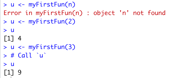
The code chunk below calls “myFirstFun(n)” and tells R to assign the results of the operation the function performs (n*n) to the variable “u”. But if we run this code as it is (with “n” in the parentheses), we will get an error (unless we have previously assigned “n” as a variable with a value that will accept the operation to be performed — so “n” needs to be a number in this case so that it can be multiplied). We do not actually want to perform the function on the letter “n” but rather, on a number that we will insert in the place of “n.”
We can apply this function by setting “n” as a number, such as 2, in the example below.
# Call the function with argument `n`
u <- myFirstFun(2)

# Call `u`
u
Once we have changed “n” to a number, R then performs this operation and saves the result to a new variable “u”. We can then ask R to tell us what “u” is, and R returns or prints the results of the function, which in this case, is the number 4 (2*2).
The image below shows the results we get if we attempt to run the function without changing the argument “n” to a number (giving us an error), and the results when we change “n” to the number “2” which assigns the result of the function (4) to “u”, or the number “3” which assigns the result of the function (now 9) to “u”.