16 Data Forensics and Cleaning: Geospatial Data

This lecture is designed to introduce you to the basics of geospatial data.

16.1 Learning Objectives

By the end of this lesson, you should:

• understand the main components of geospatial data are locations, attributes, and a coordinate reference system
• understand how geospatial data can be represented with different data models
• understand that the data structures we were already familiar with can be modified to contain spatial data.
• learn some common processes for cleaning our geospatial data

16.2 What is Geospatial Data?

Geospatial data (also known as spatial data, GIS data, and other names) is information that can be attributed to a real-world location or can relate to each other in space.

Technically, “geospatial” refers to locations on Earth, while “spatial” can be locations anywhere, including other planets or even ficticious places (like J.R.R. Tolkien’s hand-drawn maps for his novels), but quite often the terms are used interchangably.

You use geospatial data every day on your smart phone through spatially-enabled apps like Google Maps, food delivery apps, fitness trackers, weather, or games like Pokemon Go.

(geo)Spatial Data = Attributes + Locations

Location = Coordinate Reference System (CRS) + Coordinates

So…

(geo)Spatial Data = Attributes + Coordinate Reference System (CRS) + Coordinates

16.2.1 Attributes

Attributes are pieces of information about a location. For example, if I’m mapping gas stations, my attributes might be something like the price of gas, the address of the station, and the company that runs it (Shell, Arco, etc.). This isn’t the same thing as metadata, which is information about the entire dataset such as who made the data, when they made it, and how the data was created.

16.2.2 Coordinate Reference System

The earth is generally round. Maps are generally flat, with a few exceptions. If you were to try to flatten out the earth, you would create some fairly major distortions. Next time you eat an orange or a tangerine, try taking off the peel and then try to create a flat solid sheet of peel from it. You’ll end up needing to cut it or smash it to get a flat surface. The same things happens to geospatial data when we try to translate it from a round globe to a flat map. But, there are ways to minimize distortions.

A coordinate reference system (sometimes called a projection) is a set of mathematical formulas that translate measurements on a round globe to a flat piece of paper. The coordinate reference system also specifies the linear units of measure (i.e. feet, meters, decimal degrees, or something else) and a set of reference lines.

For our purposes, we can think of coordinate reference systems coming in two flavors. One is geographic coordinate systems. For simplicity’s sake, we can think of these as coordinate reference systems that apply to latitude and longitude coordinates. Projected coordinate systems translate latitude and longitude coordinates into linear units from a specified baseline and aim to reduce some aspect of the distortion introduced in the round to flat translation. (I am very much simplifying this concept so we can learn the basics without getting overwhelmed.)

To work with more than one digital spatial dataset, the coordinate reference systems must match. If they don’t match, you can transform your data into a different coordinate reference system.

16.2.3 Coordinates

Coordinates are given in the distance (in the linear units specified in the CRS) from the baselines (specified in the CRS). Coordinates can be plotted just like coordinates on a graph (cartesian coordinate system). Sometimes we refer to these as X and Y, just like a graph, but sometimes you’ll hear people refer to the cardinal directions (north, south, east, and west).

Let’s take a moment to talk about latitude and longitude. You’re probably at least a little familiar with latitude (Y) and longitude (X), but this is a special case that’s more complex than we probably initially realize. Latitude and longitude are angular measurements (with units in degrees) from a set of baselines - usually the Equator and the Greenwhich Meridian. We can plot latitude and longitude on a cartesian coordinate system, but this introduces major distortions increasing as you approach the poles. You never want to use straight latitude/longitude coordinates (commonly in North America, you’ll see data in the geographic coordinate reference system called WGS84) for an analysis. Always translate them into a projected coordinate system first. In addition, because the units are degrees, they are rather hard for us to interpret when we make measurements. How many degrees is it from the UC Davis campus to your appartment? It’s probably a very small fraction of a degree. Area measurements make even less sense. (What is a square degree and what does that look like?) Latitude/longitude coordinates are a great starting place, we just need to handle them correctly.

16.3 Geospatial Data Models

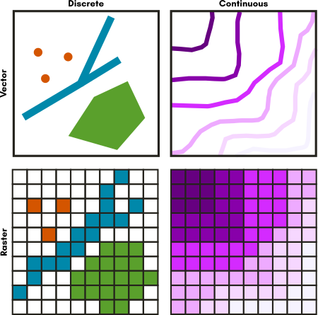
Now we have an idea of what makes data spatial, but what does spatial data look like in a computer? There are two common data models for geospatial data: Vector and Raster.

Data Model	Geometry	Example
Vector	Points	Very small things, like cities at world scale
.	Lines	Linear things, like roads at city scale
.	Polygons	Larger things that take up space, like parks at a city scale
Raster	Grid	Digital Photo

A visual table of raster vs. vector data as continuous and discrete data.

16.3.1 Vector Data

Vector data represents discrete objects in the real world with points, lines, and polygons in the dataset.

If you were to draw a map to your house for a friend, you would typically use vector data - roads would be lines, a shopping center included as an important landmark might be a rectangle of sorts, and your house might be a point (perhaps represented by a star or a house icon).

For this lecture, we will focus on point data.

16.3.2 Raster Data

Raster data represents continuous fields or discrete objects on a grid, storing measurements or category codes in each cell of the grid.

Digital photos are raster data you are already familiar with. If you zoom in far enough on a digital photo, you’ll see that photo is made up of pixels, which appear as colored squares. Pixels are cells in a regular grid and each contains the digital code that corresponds to the color that should be displayed there. Satellite images (like you see in Google Maps) are a very similar situation.

16.4 Data Structures Applied to Geospatial Data

In the lecture on Data Structures (week 6), you learned that data can be structured in a number of ways, including tabular, tree (XML and JSON), relational databases, and non-hierarchical data. All of these structures can include spatial information.

Data Structure	Example File Type	How it’s implemented
Tabular	CSV	One or more columns hold spatial data (like Latitude & Longitude)
Tree	geoJSON	Tags in the structure indicate spatial information like geometry type and vertex locations
Relational Database	PostGIS or Spatialite	One column holds the “geometry” information (vertexes & CRS)
Non-Hierarchical Relational Data	Spatial Graph Databases	Nodes have locations associated with them, edges represent flow (think: transportation networks or stream networks)

For visualization purposes, geospatial software typically show all of these data structures as a map where each entity is linked with a table of the attribute data - one row of data in the table relates to one entity on the map. So regardless of the underlying data structure, you can think of these as interactive maps like you find on Google Maps.

16.5 Cleaning Geospatial Data

What Can Go Wrong?

1. Location data isn’t usable
2. Location data is incorrect
3. Attribute data is incorrect
4. Coordinate Reference System (CRS) is improperly defined

16.5.1 Example Data

The dataset we’ll be working with as an example contains locations and attributes about lake monsters. Lake monsters are fictional creatures like sea monsters, but they live in lakes and not the ocean. The most famous lake monster is probably Nessie, who lives in Loch Ness. The dataset we’re working with today is the early stages of a now much cleaner dataset. This data came from a Wikipedia page and the locations were geocoded (a process that matches text locations with real-world locations). We’ll walk through some common processes and challenges with point data stored in a csv file.

16.5.2 Making Location Data Usable

Someone sends you a CSV file. At first glance, nothing looks amiss. There is a column for latitude and another for longitude, but how is it formatted? It’s degrees-minutes-seconds (DMS)! DMS looks like this: 34° 36’ 31.774” - 34 degrees, 36 minutes, 31.447 seconds - and sometimes people put in the symbols for degree (°), minutes (’), and seconds (“), and sometimes not. The computer can’t read this format, especially the symbols. It has to be converted to decimal degrees (DD), which looks like this: 34.60882611

To convert it, we need to know that there are 60 minutes in a degree and 60 seconds in a minute.

Decimal Degrees = Degrees + (Minutes/60) + (Seconds/3600)

34.60882611 = 34 + (36/60) + (31.447/3600)

First, we need to load the libraries we’ll need and then load the data.

# Load Libraries ----------------------------------------------------------
library("sf")

## Linking to GEOS 3.11.0, GDAL 3.5.3, PROJ 9.1.0; sf_use_s2() is TRUE

library("mapview")
library("gdtools") #makes the display... dependency of mapview but it's not loading
library("leafem") #makes the labels work... dependency of mapview but it's not loading
library("leaflet")

# Read Data ---------------------------------------------------------------

monsters.raw<-read.csv("data/lake_monsters.csv", stringsAsFactors = FALSE, encoding = "utf-8")


#Explore the data
head(monsters.raw)

##   fid field_1               Lake        Area        Country     Continent
## 1   1       1      Arenal Lagoon    Alajuela     Costa Rica North America
## 2   2       2    Bangweulu Swamp                     Zambia        Africa
## 3   3       3 Bassenthwaite Lake     England United Kingdom        Europe
## 4   4       4          Bear Lake Idaho, Utah            USA North America
## 5   5       5        Brosno Lake Tver Oblast         Russia        Europe
## 6   6       6   Bueng Khong Long   Bueng Kan       Thailand          Asia
##                          Name       lat         lon        lat_dms
## 1                     unnamed  10.49143  -84.851696 10°29?29.1304?
## 2                      Nsanga -11.14741   29.784582 -11°8?50.6760?
## 3                       Eachy  54.65279   -3.213612 54°39?10.0359?
## 4 Bear Lake Monster, Isabella  42.21721 -111.319881  42°13?1.9643?
## 5               Brosno Dragon  56.82407   31.914652 56°49?26.6520?
## 6                  Phaya Naga  18.02363  104.014360  18°1?25.0676?
##            lon_dms                                 coords_3395    lon_3395
## 1   -84°51?6.1069?  Point (-9445647.63285386 1166706.48735204)  -9445647.6
## 2    29°47?4.4935?  Point (3315604.44829715 -1240572.14607131)   3315604.4
## 3   -3°12?49.0016?   Point (-357737.60213262 7259890.14217639)   -357737.6
## 4 -111°19?11.5709? Point (-12392072.44582391 5164853.16566773) -12392072.4
## 5   31°54?52.7472?   Point (3552722.80948453 7688451.06249625)   3552722.8
## 6   104°0?51.6974?  Point (11578825.63491604 2027100.69217741)  11578825.6
##   lat_3395
## 1  1166706
## 2 -1240572
## 3  7259890
## 4  5164853
## 5  7688451
## 6  2027101

Next, we need to write some functions to deal with our specific DMS data and how its formatted.

# Functions ---------------------------------------------------------------

#This function splits up the DMS column into three columns - D, M, & S
split.dms<-function(dms.column){
  #separate the pieces of the DMS column

  variable<-do.call(rbind, args=c(strsplit(dms.column, '[°?]+'))) #makes a matrix of characters
  mode(variable)="numeric"  #assigning the data type to numeric instead of character
  dms.split<-as.data.frame(variable)
  
  split.string<-strsplit(dms.column, '[°?]+')
  
  
  #   naming the columns
  names(dms.split)<-c("D", "M", "S")
  
  return(dms.split)
}


# this function coverts a 3 column dataframe of DMS to DD, like the data created by split.dms()
decimaldegrees<-function(dms.df){
  dd<-data.frame()
  
  for (i in 1:dim(dms.df)[1]){
    if (dms.df[i, 1]>0){
      #Decimal Degrees = Degrees + (Minutes/60) + (Seconds/3600)
      dd.row<-dms.df[i,1]+(dms.df[i,2]/60)+(dms.df[i,3]/3600)
      dd<-rbind(dd, dd.row)
    } 
    else{
      #-Decimal Degrees = Degrees - (Minutes/60) - (Seconds/3600)
      dd.row<-dms.df[i,1]-(dms.df[i,2]/60)-(dms.df[i,3]/3600)
      dd<-rbind(dd, dd.row)
    }
  }
  return(dd)
}

Finally, we can process our DMS data to convert it to Decimal Degreess (DD).

#   Process Latitude
dms.split<-split.dms(monsters.raw$lat_dms)
dd<-decimaldegrees(dms.split)
monsters.df<-cbind(monsters.raw, dd)
names(monsters.df)[15]<-"lat_dd"

#   Process Longitude
dms.split<-split.dms(monsters.raw$lon_dms)
dd<-decimaldegrees(dms.split)
monsters.df<-cbind(monsters.df, dd)
names(monsters.df)[16]<-"lon_dd"

#   Look at the data
head(monsters.df)

##   fid field_1               Lake        Area        Country     Continent
## 1   1       1      Arenal Lagoon    Alajuela     Costa Rica North America
## 2   2       2    Bangweulu Swamp                     Zambia        Africa
## 3   3       3 Bassenthwaite Lake     England United Kingdom        Europe
## 4   4       4          Bear Lake Idaho, Utah            USA North America
## 5   5       5        Brosno Lake Tver Oblast         Russia        Europe
## 6   6       6   Bueng Khong Long   Bueng Kan       Thailand          Asia
##                          Name       lat         lon        lat_dms
## 1                     unnamed  10.49143  -84.851696 10°29?29.1304?
## 2                      Nsanga -11.14741   29.784582 -11°8?50.6760?
## 3                       Eachy  54.65279   -3.213612 54°39?10.0359?
## 4 Bear Lake Monster, Isabella  42.21721 -111.319881  42°13?1.9643?
## 5               Brosno Dragon  56.82407   31.914652 56°49?26.6520?
## 6                  Phaya Naga  18.02363  104.014360  18°1?25.0676?
##            lon_dms                                 coords_3395    lon_3395
## 1   -84°51?6.1069?  Point (-9445647.63285386 1166706.48735204)  -9445647.6
## 2    29°47?4.4935?  Point (3315604.44829715 -1240572.14607131)   3315604.4
## 3   -3°12?49.0016?   Point (-357737.60213262 7259890.14217639)   -357737.6
## 4 -111°19?11.5709? Point (-12392072.44582391 5164853.16566773) -12392072.4
## 5   31°54?52.7472?   Point (3552722.80948453 7688451.06249625)   3552722.8
## 6   104°0?51.6974?  Point (11578825.63491604 2027100.69217741)  11578825.6
##   lat_3395    lat_dd      lon_dd
## 1  1166706  10.49143  -84.851696
## 2 -1240572 -11.14741   29.784582
## 3  7259890  54.65279   -3.213612
## 4  5164853  42.21721 -111.319881
## 5  7688451  56.82407   31.914652
## 6  2027101  18.02363  104.014360

Another common issue with point data is that the latitude and longitude are not in any form of degrees, but instead are in a projected coordinate system with linear units (usually feet or meters). If the data doesn’t come with metadata, you may be left guessing which coordinate system it is in. With experience, you’ll get better at guessing, but sometimes the data is not usable. Our monsters dataset has latitude and longitude in the World Mercator (EPSG: 3395) projection as well. Let’s briefly look at that here, but we’ll play with that more later in this document.

monsters.df[1:10,13:16]

##       lon_3395 lat_3395    lat_dd      lon_dd
## 1   -9445647.6  1166706  10.49143  -84.851696
## 2    3315604.4 -1240572 -11.14741   29.784582
## 3    -357737.6  7259890  54.65279   -3.213612
## 4  -12392072.4  5164853  42.21721 -111.319881
## 5    3552722.8  7688451  56.82407   31.914652
## 6   11578825.6  2027101  18.02363  104.014360
## 7   -7845463.9  5433619  43.98618  -70.477001
## 8  -12704546.6  6054836  47.87777 -114.126884
## 9   -9467608.2  5128572  41.97447  -85.048971
## 10 -12525669.2  5011829  41.18707 -112.520000

Note that data preparation and cleaning is the vast majority of the work for all data, not just spatial data. All of the code we just looked at was just to get the data in a usable format. We’ll convert it to a spatial data type and map it in the next section.

16.5.3 Cleaning Location Data

Sometimes, the locations in your dataset are incorrect. This can happen for a number of reasons.

For example, it’s fairly common for data to get truncated or rounded if you open a CSV in Excel. Removing decimal places from coordinate data loses precision.

People often swap their latitude and longitude columns as well, which make data show up in the wrong cartesian coordinate, for example, (-119, 34) is a verry different location than (34, -119)… -119 is actually out of the range of latitude data and will often break your code.

Another common source of error is in the way the data was made. If data is produced by geocoding, turning an address or place name into a coordinate, the location may have been matched badly. If the data was made by an analysis process, an unexpected aspect of the data could cause problems, like a one-to-many join when you thought you had a one-to-one join in a database.

Regardless of how the errors came about, how do we find incorrect locations? Start by mapping the data and see where it lands. Is it where you expect the data to be? Sometimes you can’t tell it’s wrong because the data looks normal.

#   Convert the monsters dataframe into an SF (spatial) object
#     Note: x is the dataframe, not longitude.
#     Coordinate Reference System (CRS) - we're using lat/long here so we need WGS84 which is EPSG code 4326 - we just need to tell R what the CRS is, we don't change it this way.  If we want to change it, we need to use st_transform().
monsters.sf<-st_as_sf(x=monsters.df, 
                      coords=c("lon_dd", "lat_dd"), 
                      crs = 4326)

#     Notice we added a geometry column!
names(monsters.sf)

##  [1] "fid"         "field_1"     "Lake"        "Area"        "Country"    
##  [6] "Continent"   "Name"        "lat"         "lon"         "lat_dms"    
## [11] "lon_dms"     "coords_3395" "lon_3395"    "lat_3395"    "geometry"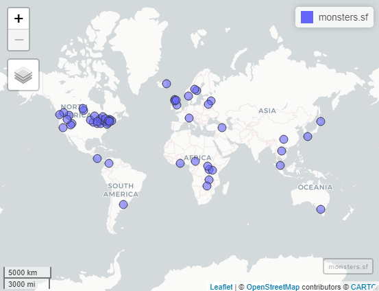

#     Plot a map
mapview(monsters.sf)

This is a screen capture of the output for the mapview function. Running this code in a regular R session (i.e. not in knitr or bookdown like we need to for this reader) will make an interactive map.

In the interactive version of this map, you can pan and zoom to different areas to see more detail. Clicking on a point will open a popup with attribute information.

First impressions: This map looks good! The points are all on land masses, none in the ocean. Let’s see if they are on the correct continent…

mapview(monsters.sf, zcol="Continent", legend= TRUE)

Map of monster locations by continent

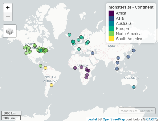
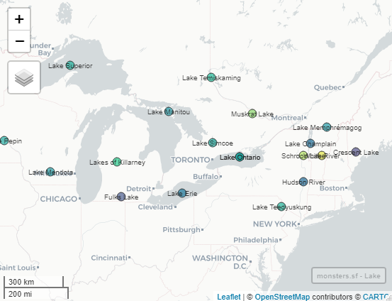
It’s hard to see, but there’s a point in Michigan that’s the wrong color for North America!

Map of monster locations by continent zoomed in to the Great Lakes

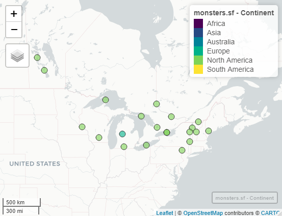
Whoops! Lakes of Killarney isn’t in Michigan! That point should be in Ireland! If we zoom in, we can see why the geocoder got confused. The lake names are very similar.

16.5.4 Cleaning Attribute Data

Attribute data can be proofed in much the same way tabular data can be proofed. You can look at the statistical properties of numeric data or the unique entities in a list of categorical variables to see if any values are odd or out of place.

With spatial data, we can also map the data and visualize it by attribute values to see if anything is out of place spatially. Labels are another helpful tool. Sometimes cleaning attributes uncovers issues with the locations.

Let’s make sure the lake names match the lakes the points are in. We’ll make a map and if you zoom in enough, the lake names will appear in the background map data.

my.label.options<-labelOptions(clickable=TRUE) #makes a popup with attribute information

map.lakename<-mapview(monsters.sf, zcol="Lake", legend= FALSE)
labels.lakename<-addStaticLabels(map.lakename, 
                                 label=monsters.sf$Lake,
                                 labelOption=my.label.options)
labels.lakename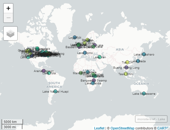

Map of monster locations by lake name zoomed in to the Great Lakes

Map of monster locations by lake name zoomed in to the Great Lakes

And for fun, let’s look at the monster names:

map.monstername<-mapview(monsters.sf, zcol="Name", legend= FALSE)
labels.monstername<-addStaticLabels(map.monstername, 
                                 label=monsters.sf$Name,
                                 labelOption=my.label.options)
labels.monstername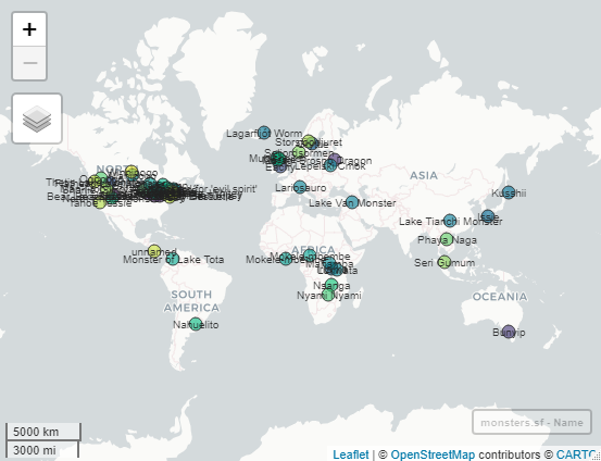

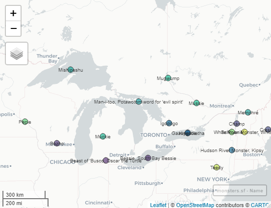
Map of monster locations by monster name zoomed in to the Great Lakes

Map of monster locations by monster name zoomed in to the Great Lakes

Yikes! That needs some clean-up too! The name column is missing some names and some records have extra information in them.

16.5.5 Checking Coordinate Reference Systems

“Why is my California data showing up in Arizona?” is a common question UC Davis researchers ask on the Geospatial email list. Why does this happen? It’s usually because the CRS for their data is impropperly defined. Someone changed the defnition but didn’t reproject the data (the mathematical process of switching CRSs). Using the wrong CRS will often shift data just enough to look really funny on a map, but sometimes it won’t show up at all.

“Why don’t my datasets line up in my map?” Again, it’s your CRS. In this case, they could be correct for all of the datasets you’re using, but each dataset has a different CRS. You can think of CRSs as different dimensions in your favorite SciFi story. Sometimes you can see the other person in the other dimension (CRS), but usually they are too different and you’re nowhere near each other. Datasets have to have the same CRS to make a map or do any analysis.

Our data came with lat/long data in another coordinate reference system - EPSG 3395 “World Mercator”, a world projection centered on Europe. Notice how the coordinates look very different from the lat/long coordinates in EPSG 4326 “WGS 84”

monsters.df[1:10,13:16]

##       lon_3395 lat_3395    lat_dd      lon_dd
## 1   -9445647.6  1166706  10.49143  -84.851696
## 2    3315604.4 -1240572 -11.14741   29.784582
## 3    -357737.6  7259890  54.65279   -3.213612
## 4  -12392072.4  5164853  42.21721 -111.319881
## 5    3552722.8  7688451  56.82407   31.914652
## 6   11578825.6  2027101  18.02363  104.014360
## 7   -7845463.9  5433619  43.98618  -70.477001
## 8  -12704546.6  6054836  47.87777 -114.126884
## 9   -9467608.2  5128572  41.97447  -85.048971
## 10 -12525669.2  5011829  41.18707 -112.520000

#   Let's make our World Mercator data spatial so we can explore its CRS
monsters.sf.3395<-st_as_sf(x=monsters.df, 
                      coords=c("lon_3395", "lat_3395"), 
                      crs = 3395)

#   st_crs tells us what the CRS is in well known text (WKT) and EPSG (if it's avaialble)
st_crs(monsters.sf)

## Coordinate Reference System:
##   User input: EPSG:4326 
##   wkt:
## GEOGCRS["WGS 84",
##     ENSEMBLE["World Geodetic System 1984 ensemble",
##         MEMBER["World Geodetic System 1984 (Transit)"],
##         MEMBER["World Geodetic System 1984 (G730)"],
##         MEMBER["World Geodetic System 1984 (G873)"],
##         MEMBER["World Geodetic System 1984 (G1150)"],
##         MEMBER["World Geodetic System 1984 (G1674)"],
##         MEMBER["World Geodetic System 1984 (G1762)"],
##         MEMBER["World Geodetic System 1984 (G2139)"],
##         ELLIPSOID["WGS 84",6378137,298.257223563,
##             LENGTHUNIT["metre",1]],
##         ENSEMBLEACCURACY[2.0]],
##     PRIMEM["Greenwich",0,
##         ANGLEUNIT["degree",0.0174532925199433]],
##     CS[ellipsoidal,2],
##         AXIS["geodetic latitude (Lat)",north,
##             ORDER[1],
##             ANGLEUNIT["degree",0.0174532925199433]],
##         AXIS["geodetic longitude (Lon)",east,
##             ORDER[2],
##             ANGLEUNIT["degree",0.0174532925199433]],
##     USAGE[
##         SCOPE["Horizontal component of 3D system."],
##         AREA["World."],
##         BBOX[-90,-180,90,180]],
##     ID["EPSG",4326]]

st_crs(monsters.sf.3395)

## Coordinate Reference System:
##   User input: EPSG:3395 
##   wkt:
## PROJCRS["WGS 84 / World Mercator",
##     BASEGEOGCRS["WGS 84",
##         ENSEMBLE["World Geodetic System 1984 ensemble",
##             MEMBER["World Geodetic System 1984 (Transit)"],
##             MEMBER["World Geodetic System 1984 (G730)"],
##             MEMBER["World Geodetic System 1984 (G873)"],
##             MEMBER["World Geodetic System 1984 (G1150)"],
##             MEMBER["World Geodetic System 1984 (G1674)"],
##             MEMBER["World Geodetic System 1984 (G1762)"],
##             MEMBER["World Geodetic System 1984 (G2139)"],
##             ELLIPSOID["WGS 84",6378137,298.257223563,
##                 LENGTHUNIT["metre",1]],
##             ENSEMBLEACCURACY[2.0]],
##         PRIMEM["Greenwich",0,
##             ANGLEUNIT["degree",0.0174532925199433]],
##         ID["EPSG",4326]],
##     CONVERSION["World Mercator",
##         METHOD["Mercator (variant A)",
##             ID["EPSG",9804]],
##         PARAMETER["Latitude of natural origin",0,
##             ANGLEUNIT["degree",0.0174532925199433],
##             ID["EPSG",8801]],
##         PARAMETER["Longitude of natural origin",0,
##             ANGLEUNIT["degree",0.0174532925199433],
##             ID["EPSG",8802]],
##         PARAMETER["Scale factor at natural origin",1,
##             SCALEUNIT["unity",1],
##             ID["EPSG",8805]],
##         PARAMETER["False easting",0,
##             LENGTHUNIT["metre",1],
##             ID["EPSG",8806]],
##         PARAMETER["False northing",0,
##             LENGTHUNIT["metre",1],
##             ID["EPSG",8807]]],
##     CS[Cartesian,2],
##         AXIS["(E)",east,
##             ORDER[1],
##             LENGTHUNIT["metre",1]],
##         AXIS["(N)",north,
##             ORDER[2],
##             LENGTHUNIT["metre",1]],
##     USAGE[
##         SCOPE["Very small scale conformal mapping."],
##         AREA["World between 80°S and 84°N."],
##         BBOX[-80,-180,84,180]],
##     ID["EPSG",3395]]

#   Check to see if they are identical, returning a logical vector
identical(st_crs(monsters.sf),
          st_crs(monsters.sf.3395))

## [1] FALSE

16.6 Conclusions

We’ve learned some of the basics of geospatial data. We learned that the main components of geospatial data are locations, attributes, and a coordinate reference system. We saw how geospatial data can be represented with different data models, but we focused on point vector data. We learned that the data structures we were already familiar with can be modified to contain spatial data. And finally, we looked at some common processes for cleaning our geospatial data.

This was a lot to cover, but we just scratched the surface of all your can do with geospatial data science! If you want to learn more, UC Davis has some fantastic introductory classes for GIS (Geographic Information Systems/Science) and Remote Sensing (working satelite data and air photos).

16.7 Optional Further Reading

1. Bolstad, P. 2019. GIS Fundamentals: A first text on geographic information systems. Sixth Edition. XanEdu. Ann Arbor, MI. 764 pp.
2. Sutton, T., O. Dassau, & M. Sutton. 2021. A Gentle Introduction to GIS. https://docs.qgis.org/3.16/en/docs/gentle_gis_introduction/preamble.html (accessed on 2021-02-11)

An, Weihua, and Yu-Hsin Liu. 2016. “Keyplayer: An R Package for Locating Key Players in Social Networks.” The R Journal 8 (1): 257. https://doi.org/10.32614/RJ-2016-018.

Balaban, Alexandru T. 1985. “Applications of Graph Theory in Chemistry.” Journal of Chemical Information and Modeling 25 (3): 334–43. https://doi.org/10.1021/ci00047a033.

Bassett, Danielle S., and Olaf Sporns. 2017. “Network Neuroscience.” Nature Neuroscience 20 (3): 353–64. https://doi.org/10.1038/nn.4502.

Fan, Chao, and Ali Mostafavi. 2019. “A Graph-Based Method for Social Sensing of Infrastructure Disruptions in Disasters.” Computer-Aided Civil and Infrastructure Engineering 34 (12): 1055–70. https://doi.org/10.1111/mice.12457.

Kadushin, Charles. 2012. Understanding Social Networks: Theories, Concepts, and Findings. New York, NY: Oxford University Press.

Krebs, Valdis E. 2002. “Mapping Networks of Terrorist Cells.” Connections 24 (3): 43–52.

Moreno, Jacob L. 1953. “Who Shall Survive?: Foundations of Sociometry, Group Psychotherapy and Sociodrama.” In. Beacon, N.Y.: Beacon House Inc.

Page, Lawrence. 2001. Method for node ranking in a linked database. US6285999B1, issued September 2001. https://patents.google.com/patent/US6285999/en.

Robins, Garry, Pip Pattison, Yuval Kalish, and Dean Lusher. 2007. “An Introduction to Exponential Random Graph (p*) Models for Social Networks.” Social Networks, Special Section: Advances in Exponential Random Graph (p*) Models, 29 (2): 173–91. https://doi.org/10.1016/j.socnet.2006.08.002.

Robins, Garry, Tom Snijders, Peng Wang, Mark Handcock, and Philippa Pattison. 2007. “Recent Developments in Exponential Random Graph (p*) Models for Social Networks.” Social Networks, Special Section: Advances in Exponential Random Graph (p*) Models, 29 (2): 192–215. https://doi.org/10.1016/j.socnet.2006.08.003.

Wasserman, Stanley, and Katherine Faust. 1994. Social Network Analysis: Methods and Applications. Cambridge, UK: Cambridge University Press.