4  ggplot2

As you have seen so far in this workshop, R has some useful tools for visualizing spatial data built in and there are packages that you can work with to make maps that are more refined. Next we’ll talk about the ggplot2 package so you can compare and contrast three of the most popular ways to make maps in R.

ggplot2 (commonly referred to as “ggplot”) is a popular package for plotting data in R. It has been extended to work with spatial data. Like tmap, it also uses the concepts of a Grammar of Graphics to layer data as well as visualization rules. ggplot is a big topic that could be its own workshop, so today we’ll cover the basics so you can learn more on your own if this sparks your interest.

A common point of confusion is the difference between ggplot and ggmap. ggmap is another popular package for making maps in R that extends the ggplot2 concept. ggmap assumes you want to use a basemap with every plot. We will focus on ggplot in this workshop.

4.1 Simple Map

First, we load the libraries we’ll need:

  #install.packages("ggplot2")
  library("ggplot2")

Warning: package 'ggplot2' was built under R version 4.4.3

  library(ggspatial)

Warning: package 'ggspatial' was built under R version 4.4.3

Grammar of Graphics tools typically follow a pattern: first you indicate which data you want to work with, then you indicate the way the data should be styled. Let’s map the states data to see a basic no-frills example:

  ggplot(states) +      #indicate which data to plot
    geom_sf()           #use the default style for sf objects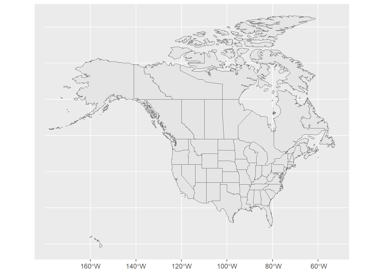

4.2 Multiple Layers

With ggplot2, if we want to add multiple layers to the map, we can think of each layer as a separate map that we stack together. For our map, we’ll first make the layer that contains the states, then we’ll add a layer that contains the lakes, then a final layer that contains the monsters.

  aoi <- st_bbox(c(xmin = -96, xmax = -73, ymax = 50, ymin = 40), crs = st_crs(4326))
  
  ggplot() +
    
    geom_sf(data = states) +        #plot the states
    
    geom_sf(data = lakes) +         #plot the lakes and make them blue
    
    geom_sf(data = monsters) +      #plot the monsters
    
    coord_sf(                       #set the zoom based on our AOI bounding box
       xlim=c(aoi[1], aoi[3]), 
       ylim=c(aoi[2], aoi[4]))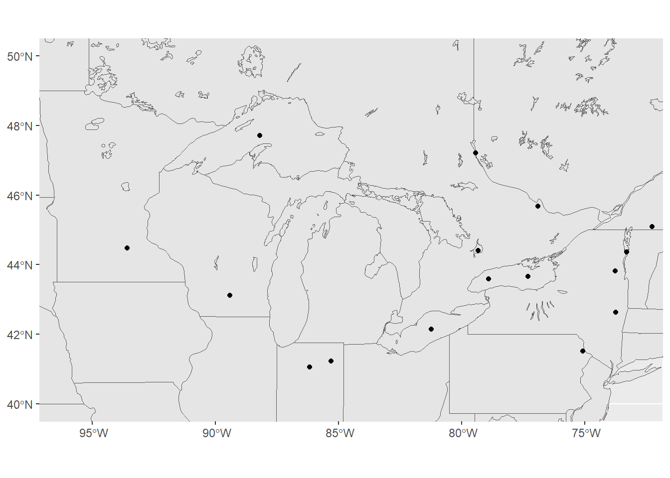

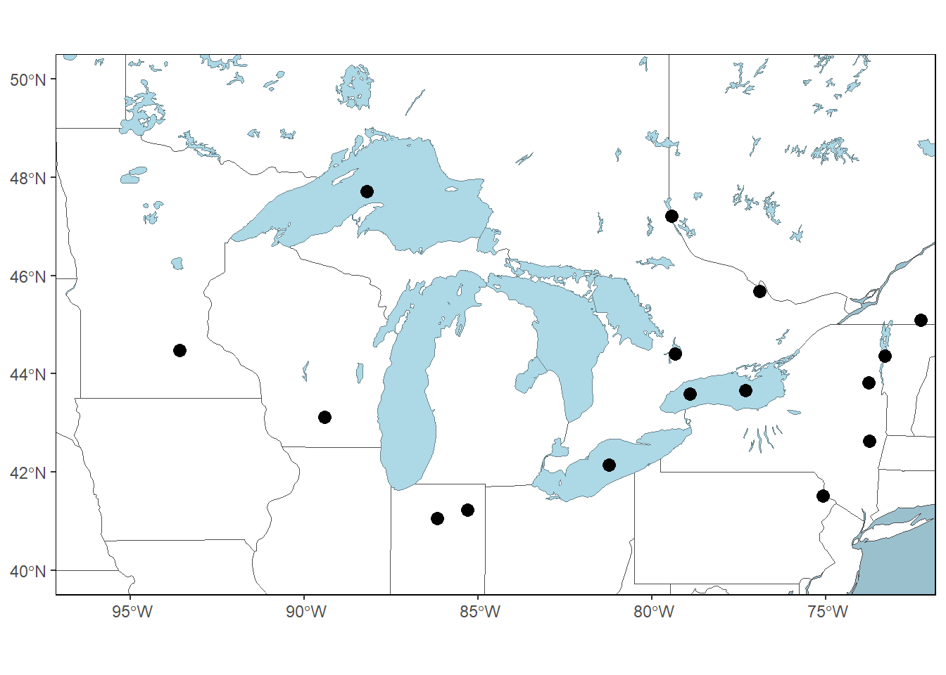
4.3 Styling

The goal of styling our data is to help it communicate better. Dots on top of state outlines are definitely difficult to understand. Let’s change the plotting arguments to make something more readable and to fit the story we want to tell.

  gg_monsters <- ggplot() +     #assign the results of the plot to a variable
  
  geom_sf(data = states,
          fill = "white",       #fill the states with white
          color = "gray30") +   #make the outline a dark gray
  
  geom_sf(                      
    data = lakes, 
    fill = "lightblue",         #fill the lakes with blue
    color = "lightblue4") +     #make the outline a gray-blue
  
  geom_sf(data = monsters,
          size = 3              #make the points larger
          ) +               
  
  coord_sf(                     
    xlim=c(aoi[1], aoi[3]), 
    ylim=c(aoi[2], aoi[4]))

  ocean_color <- "lightblue3"     #pick a color for the ocean

  gg_monsters +                   #add theme parameters to the plot & remove lines
    theme(
      panel.background = element_rect(fill = ocean_color, color = ocean_color),
      panel.grid.major = element_line(color = ocean_color),
      panel.grid.minor = element_line(color = ocean_color),
      panel.border = element_rect(color = "black", fill = NA)   #add a black neatline
      )

4.4 Add Text Labels

Let’s add some text labels so we know what the names of each of the monsters are. We can just update the last line of the code we wrote above, adding the labeling details.

  gg_monsters +                   
  theme(
    panel.background = element_rect(fill = ocean_color, color = ocean_color),
    panel.grid.major = element_line(color = ocean_color),
    panel.grid.minor = element_line(color = ocean_color),
    panel.border = element_rect(color = "black", fill = NA)
  ) +
  geom_sf_text(data=monsters, aes(label = Name), nudge_y = -.3) #add the label text and nudge them down so the letters aren't on top of the point

Warning in st_point_on_surface.sfc(sf::st_zm(x)): st_point_on_surface may not
give correct results for longitude/latitude data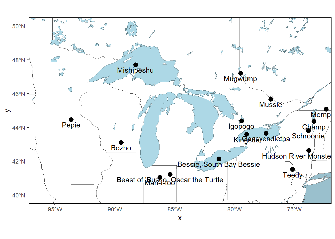

Labeling of points is challenging for all of the methods we’ve looked at. ggplot2 has some options to avoid label collisions (overlaps) that you you can explore more on your own. If you want finer label placement control, export a pdf and edit it in a vector illustration software like Inkscape or Adobe Illustrator.

4.5 North Arrow & Scale Bar

ggplot2 does not come with the ability to add map elements like a north arrow or scale bar to your map, but we can add this capability with another package: ggspatial.

  gg_monsters +                   #add theme parameters to the plot & remove lines
  theme(
    panel.background = element_rect(fill = ocean_color, color = ocean_color),
    panel.grid.major = element_line(color = ocean_color),
    panel.grid.minor = element_line(color = ocean_color),
    panel.border = element_rect(color = "black", fill = NA)
  ) +
  geom_sf_text(data=monsters, aes(label = Name), nudge_y = -.3)+
  annotation_scale(location = "bl", pad_x = unit(2, "cm"))+         #add the scale bar and move it over a little to the right
  annotation_north_arrow(location = "bl", which_north = "grid")     #add the north arrow

Warning in st_point_on_surface.sfc(sf::st_zm(x)): st_point_on_surface may not
give correct results for longitude/latitude data

Scale on map varies by more than 10%, scale bar may be inaccurate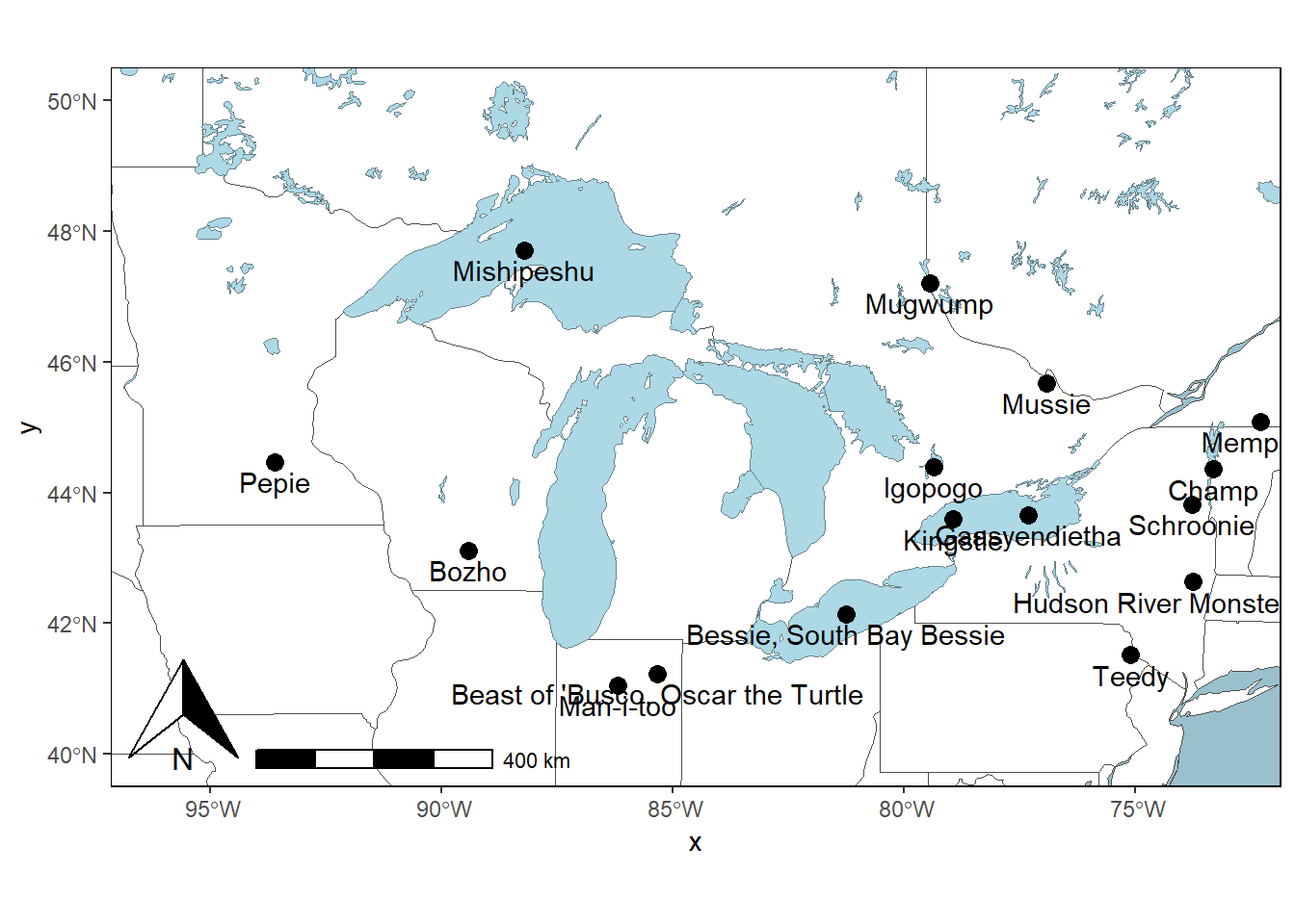

This map is far from beautiful, but it’s a good first draft. If you like ggplot2, there’s a lot more you can learn about refining placement and style options, but you’ve seen the basics to know what’s possible and you’ve got a starting point to learn more on your own.

5 Ready-Made Tile Services

ggmap is another popular package for making maps in R that extends the ggplot2 concept. ggmap assumes you want to use a basemap with every plot.

Remember that even if a tile service makes a dataset easy to use, you still need to comply with the terms of service for that specific dataset.

Unfortunately, it seems that the current version of ggmap requires you to have a Google API Key to access even non-Google tiles. That’s outside the scope of this workshop, but there is documentation on the internet for how to use this tool to build ggplot2 maps on top of a basemaps.

5.1 Summary

We’ve seen that we can build a map in layers using ggplot2 in a similar manner to the workflow we used in the base plot() and tmap workflow. ggplot2 is an entire universe of plot creation with many options for fine control and attractive themes that you can explore. It has perhaps the steepest learning curve, but also has big rewards if you have the patience to stick with it.