    #install.packages("tmap")
    library("tmap")
Warning: package 'tmap' was built under R version 4.4.3tmap is a popular package for making maps. It uses the concepts of a Grammar of Graphics to layer data as well as visualization rules. If you’re familiar with the ggplot2 package, this will feel similar. If you’re not familiar with ggplot2 (or not a fan), that’s ok because tmap uses layers in much the same way we just built maps using the base R plot() function.
First, we load the libraries we’ll need:
#install.packages("tmap")
library("tmap")Warning: package 'tmap' was built under R version 4.4.3Grammar of Graphics tools typically follow a pattern: first you indicate which data you want to work with, then you indicate the way the data should be styled. Let’s map the states data to see a basic no-frills example:
    tm_shape(states) +    #the data we want to map
    tm_polygons()         #style the data using the defaults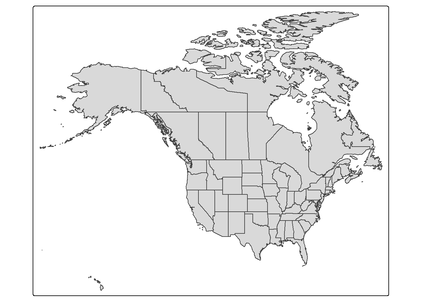
With tmap, if we want to add multiple layers to the map, we can think of each layer as a separate map that we stack together. For our map, we’ll first make the layer that contains the states, then we’ll add a layer that contains the lakes, then a final layer that contains the monsters.
  map_states <- tm_shape(states) +
    tm_polygons()

  map_lakes <- map_states +         #start with the states map
    tm_shape(lakes) +               #add the lakes data
    tm_polygons()                   #style the lakes data

  map_monsters <- map_lakes +       #start with the lakes map
    tm_shape(monsters) +            #add the monsters data
    tm_dots()                       #style the monsters data

  map_monsters                      #call the map variable to plot the map inside it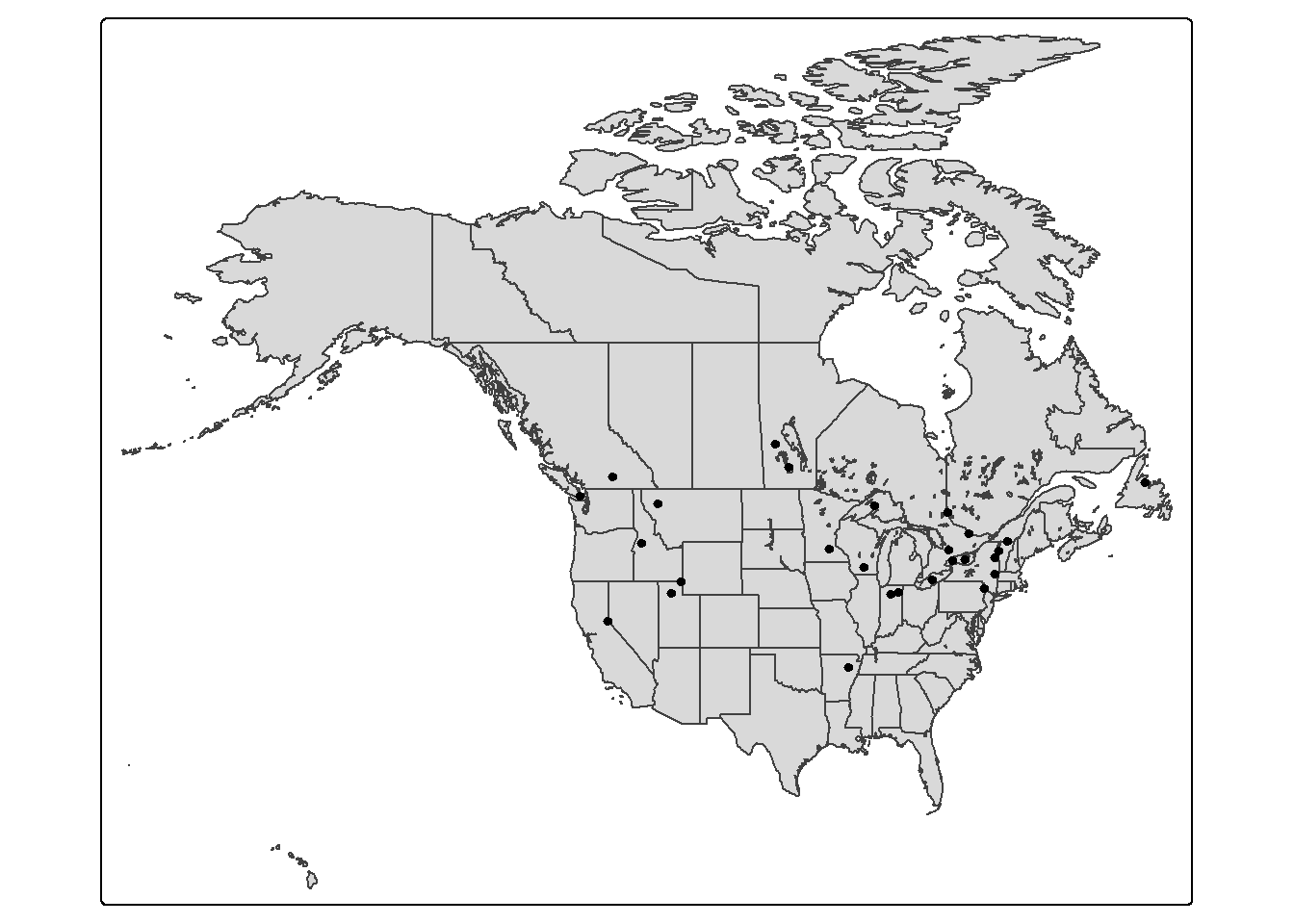
The goal of styling our data is to help it communicate better. Dots on top of state outlines are definitely difficult to understand. Let’s change the plotting arguments to make something more readable and to fit the story we want to tell.
  #create a bounding box object for the zoom area of our map
  aoi <- st_bbox(c(xmin = -96, xmax = -73, ymax = 50, ymin = 40), crs = st_crs(4326))


    map_states <-
      tm_shape(states,
         bbox = aoi) +                    #set the extend for the map

    tm_polygons(
      fill="white",                     #fill the polygons with white
      col="gray30") +                   #make the outline dark gray
    tm_layout(bg.color="lightblue3")    #set the background color with the layout options


    map_lakes <- map_states +
      tm_shape(lakes) +
      tm_polygons(
        fill = "lightblue",               #fill the polygons with light blue
        col="lightblue4"                  #make the outline a darker blue
      )

  map_monsters <- map_lakes +
    tm_shape(monsters) +
    tm_dots(size=.5)                    #set the size of the points

map_monsters 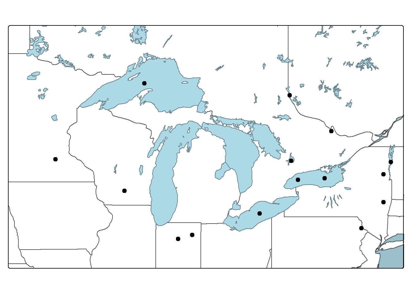
Let’s add some text labels so we know what the names of each of the monsters are.
  #create a bounding box object for the zoom area of our map
  aoi <- st_bbox(c(xmin = -96, xmax = -73, ymax = 50, ymin = 40), crs = st_crs(4326))


    map_states <-
      tm_shape(states,
         bbox = aoi) +

    tm_polygons(
      fill="white",
      col="gray30") +
    tm_layout(bg.color="lightblue3")


    map_lakes <- map_states +
    tm_shape(lakes) +
    tm_polygons(
      fill = "lightblue",
      col="lightblue4"
      )

  map_monsters <- map_lakes +
    tm_shape(monsters) +
    tm_dots(size=.5) +

    tm_text("Name")             #create labels, specifying the column to use

map_monsters 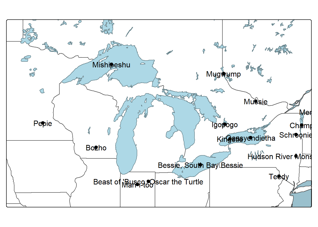
Labeling of points is challenging for tmap. It doesn’t have a way to avoid label collisions (overlaps) and the placement options don’t really do much to avoid labels running over the symbols. I also haven’t found much guidance on placing the labels. Most of the tutorials avoid this problem by labeling polygons where the exact placement isn’t a concern. Like the discussion of plot(), this map would benefit from moving the labels by hand. Export a pdf and edit it in a vector illustration software like Inkscape or Adobe Illustrator.
One big benefit of the tmap workflow is the built in option to add norh arrows and scale bars. Adding them in is super simple and if you’re happy with the defaults, it’s pretty quick. We’ll put ours in the lower left corner where they won’t cover up our monster points. Also, we’re adding these to the last layer of the map we built so that the arrow and scale bar don’t get covered up by anything else. (Note I’m taking out the labels because they are messy.)
  #create a bounding box object for the zoom area of our map
  aoi <- st_bbox(c(xmin = -96, xmax = -73, ymax = 50, ymin = 40), crs = st_crs(4326))


    map_states <-
      tm_shape(states,
         bbox = aoi) +

    tm_polygons(
      fill="white",
      col="gray30") +
    tm_layout(bg.color="lightblue3")


    map_lakes <- map_states +
    tm_shape(lakes) +
    tm_polygons(
      fill = "lightblue",
      col="lightblue4"
      )

  map_monsters <- map_lakes +
    tm_shape(monsters) +
    tm_dots(size=.5) +

    tm_compass(position=c("left", "bottom")) +     #add the north arrow (compass rose)
    tm_scalebar(position=c("left", "bottom"))      #add the scale bar


map_monsters 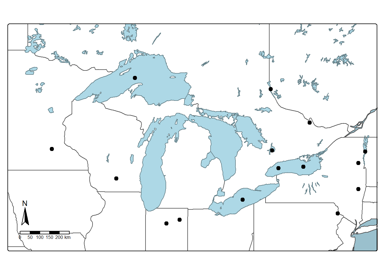
Another benefit of the tmap workflow is the easy availability of using tile services (commonly known as “basemaps” but people use that term to mean so many other things as well). Tile services are continuous map layers that are stored in square chunks (tiles) so you only need to load the part of the world in your area of interest. One tile service that many people are familiar with is Google Maps, but open data like OpenStreetMap is also available as a tile service.
Remember that even if a tile service makes a dataset easy to use, you still need to comply with the terms of service for that specific dataset.
Let’s replace our base layers (states and lakes) with the default basemap.
  #create a bounding box object for the zoom area of our map
  aoi <- st_bbox(c(xmin = -96, xmax = -73, ymax = 50, ymin = 40), crs = st_crs(4326))


      map_monsters <-
        tm_basemap() +                       #start with the default base map
      tm_shape(monsters, bbox = aoi) +     #move the bounding box parameter here
      tm_dots(size=.5) +

      tm_compass(position=c("left", "bottom")) +
      tm_scalebar(position=c("left", "bottom"))


map_monsters 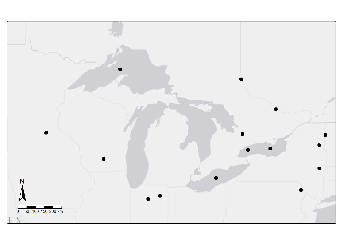
What about a base layer with some more color or labels? Let’s add the OpenStreetMap tile service.
  #create a bounding box object for the zoom area of our map
  aoi <- st_bbox(c(xmin = -96, xmax = -73, ymax = 50, ymin = 40), crs = st_crs(4326))


      map_monsters <-
        tm_basemap("OpenStreetMap") +                       #start with the default base map
      tm_shape(monsters, bbox = aoi) +
      tm_dots(size=.5) +

      tm_compass(position=c("left", "bottom")) +
      tm_scalebar(position=c("left", "bottom"))


map_monsters 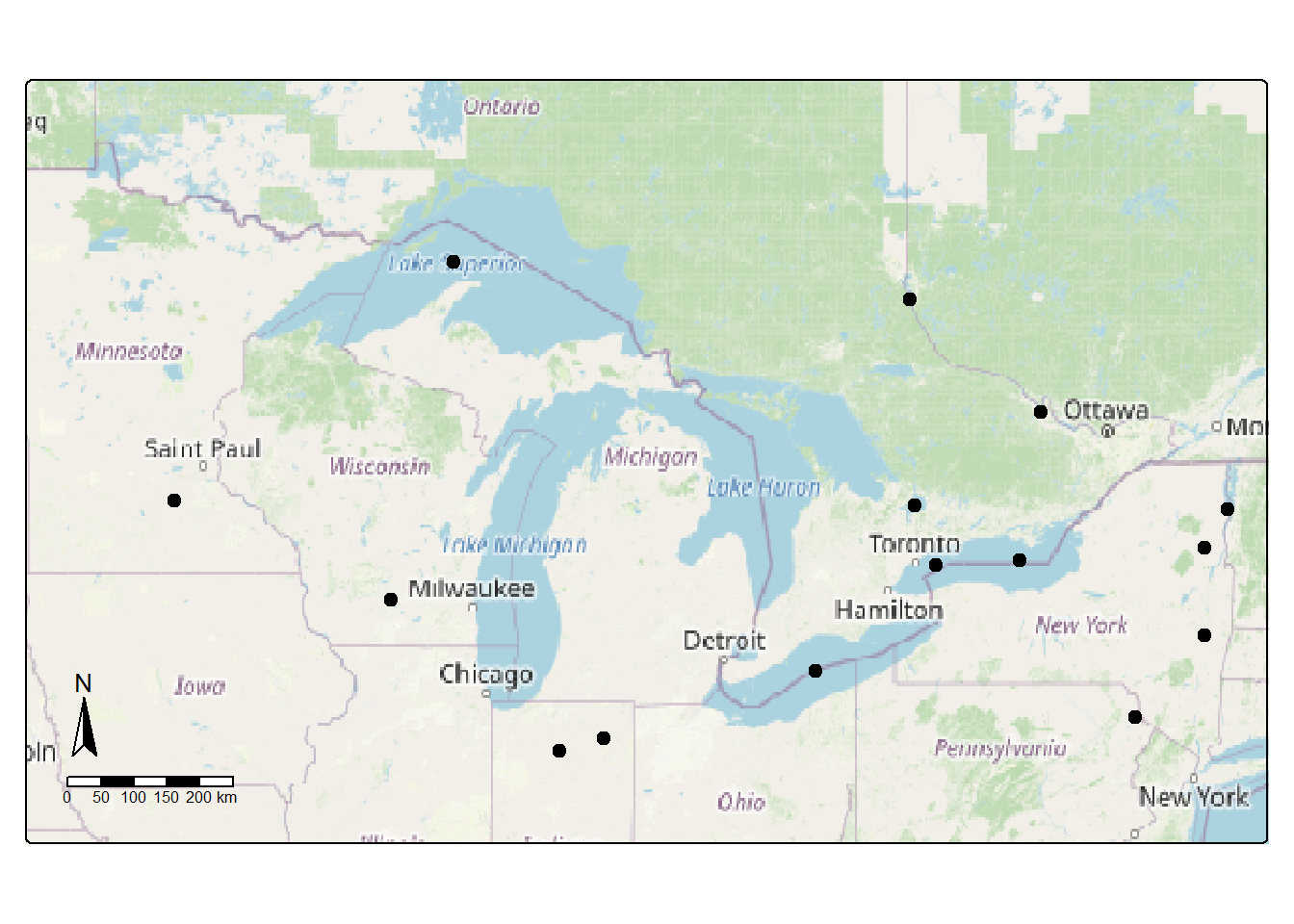
Being able to pan and zoom around a plot is a useful tool for understanding your data or the results of an analysis. tmap makes this relatively easy with the tmap_leaflet() function. Let’s plot our monster data on the default basemap. The pattern of the code should look familiar: set up the map, building up layers from the bottom, and then plot the map.
  #create a bounding box object for the zoom area of our map
  aoi <- st_bbox(c(xmin = -96, xmax = -73, ymax = 50, ymin = 40), crs = st_crs(4326))

leaflet_map =
  tm_shape(monsters, bbox = aoi) +      #add the monster data
  tm_dots(size=.5)                      #style the monster data

tmap_leaflet(leaflet_map, show = TRUE)  #plot the monster data
Notice the source information for the basemap printed in the lower right corner of the map. If you want to publish this map, you’ll need to check the Terms of Service for this data source.
Try zooming out and panning around the world to see more lake monster locations in context. You can change your basemap like we did earlier in the workshop with a parameter like tm_basemap("OpenStreetMap") when you define your map contents.
We’ve seen that we can build a map in layers using tmap in a similar manner to the workflow we used in the base plot() workflow. tmap has more built-in features for composing maps and finer control over some aspects of maps like north arrows and scale bars. It also has built-in base map tools which makes making a map quick. But tmap still doesn’t have an easy way to deal with label placement.