4 Automating Tasks

By now, you’ve learned all of the basic skills necessary to explore a data set in R. The focus of this chapter is how to organize your code so that it’s concise, clear, and easy to automate. This will help you and your collaborators avoid tedious, redundant work, reproduce results efficiently, and run code in specialized environments for scientific computing, such as high-performance computing clusters.

Learning Objectives

• Create code that only runs when a condition is satisfied
• Create custom functions in order to organize and reuse code
• Run code repeatedly in a for-loop
• Describe the different types of loops and how to choose between them

4.1 Conditional Expressions

Sometimes you’ll need code to do different things, depending on a condition. If-statements provide a way to write conditional code.

For example, suppose we want to greet one person differently from the others:

name = "Nick"
if (name == "Nick") {
   # If name is Nick:
   message("We went down the TRUE branch")
   msg = "Hi Nick, nice to see you again!"
} else {
   # Anything else:
   msg = "Nice to meet you!"
}

## We went down the TRUE branch

Indent code inside of the if-statement by 2 or 4 spaces. Indentation makes your code easier to read.

The condition in an if-statement has to be a scalar:

name = c("Nick", "Susan")
if (name == "Nick") {
   msg = "Hi Nick!"
} else {
   msg = "Nice to meet you!"
}

## Error in if (name == "Nick") {: the condition has length > 1

You can chain together if-statements:

name = "Susan"
if (name == "Nick") {
   msg = "Hi Nick, nice to see you again!"
} else if (name == "Peter") {
   msg = "Go away Peter, I'm busy!"
} else {
   msg = "Nice to meet you!"
}
msg

## [1] "Nice to meet you!"

If-statements return the value of the last expression in the evaluated block:

name = "Tom"
msg = if (name == "Nick") {
   "Hi Nick, nice to see you again!"
} else {
   "Nice to meet you!"
}
msg

## [1] "Nice to meet you!"

Curly braces { } are optional for single-line expressions:

name = "Nick"
msg = if (name == "Nick") "Hi Nick, nice to see you again!" else
   "Nice to meet you!"
msg

## [1] "Hi Nick, nice to see you again!"

But you have to be careful if you don’t use them:

# NO GOOD:
msg = if (name == "Nick")
   "Hi Nick, nice to see you again!"
else
   "Nice to meet you!"

## Error: <text>:4:1: unexpected 'else'
## 3:    "Hi Nick, nice to see you again!"
## 4: else
##    ^

The else block is optional:

msg = "Hi"
name = "Tom"
if (name == "Nick")
   msg = "Hi Nick, nice to see you again!"
msg

## [1] "Hi"

When there’s no else block, the value of the else block is NULL:

name = "Tom"
msg = if (name == "Nick")
   "Hi Nick, nice to see you again!"
msg

## NULL

4.2 Functions

The main way to interact with R is by calling functions, which was first explained way back in Section 1.2.4. Since then, you’ve learned how to use many of R’s built-in functions. This section explains how you can write your own functions.

To start, let’s briefly review what functions are, and some of the jargon associated with them. It’s useful to think of functions as factories: raw materials (inputs) go in, products (outputs) come out. We can also represent this visually:

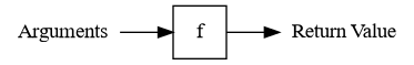
Programmers use several specific terms to describe the parts and usage of functions:

• Parameters are placeholder variables for inputs.
  • Arguments are the actual values assigned to the parameters in a call.
• The return value is the output.
• The body is the code inside.
• Calling a function means using a function to compute something.

Almost every command in R is a function, even the arithmetic operators and the parentheses! You can view the body of a function by typing its name without trailing parentheses (in contrast to how you call functions). The body of a function is usually surrounded by curly braces {}, although they’re optional if the body only contains one line of code. Indenting code inside of curly braces by 2-4 spaces also helps make it visually distinct from other code.

For example, let’s look at the body of the append function, which appends a value to the end of a list or vector:

append

## function (x, values, after = length(x)) 
## {
##     lengx <- length(x)
##     if (!after) 
##         c(values, x)
##     else if (after >= lengx) 
##         c(x, values)
##     else c(x[1L:after], values, x[(after + 1L):lengx])
## }
## <bytecode: 0x5612956fee98>
## <environment: namespace:base>

Don’t worry if you can’t understand everything the append function’s code does yet. It will make more sense later on, after you’ve written a few functions of your own.

Many of R’s built-in functions are not entirely written in R code. You can spot these by calls to the special .Primitive or .Internal functions in their code.

For instance, the sum function is not written in R code:

sum

## function (..., na.rm = FALSE)  .Primitive("sum")

The function keyword creates a new function. Here’s the syntax:

function(parameter1, parameter2, ...) {
  # Your code goes here

  # The result goes here
}

A function can have any number of parameters, and will automatically return the value of the last line of its body.

A function is a value, and like any other value, if you want to reuse it, you need to assign it to variable. Choosing descriptive variable names is a good habit. For functions, that means choosing a name that describes what the function does. It often makes sense to use verbs in function names.

Let’s write a function that gets the largest values in a vector. The inputs or arguments to the function will be the vector in question and also the number of values to get. Let’s call these vec and n, respectively. The result will be a vector of the n largest elements. Here’s one way to write the function:

get_largest = function(vec, n) {
  sorted = sort(vec, decreasing = TRUE)
  head(sorted, n)
}

The name of the function, get_largest, describes what the function does and includes a verb. If this function will be used frequently, a shorter name, such as largest, might be preferable (compare to the head function).

Any time you write a function, the first thing you should do afterwards is test that it actually works. Let’s try the get_largest function on a few test cases:

x = c(1, 10, 20, -3)
get_largest(x, 2)

## [1] 20 10

get_largest(x, 3)

## [1] 20 10  1

y = c(-1, -2, -3)
get_largest(y, 2)

## [1] -1 -2

z = c("d", "a", "t", "a", "l", "a", "b")
get_largest(z, 3)

## [1] "t" "l" "d"

Notice that the parameters vec and n inside the function do not exist as variables outside of the function:

vec

## Error in eval(expr, envir, enclos): object 'vec' not found

In general, R keeps parameters and variables you define inside of a function separate from variables you define outside of a function. You can read more about the specific rules for how R searches for variables in Section 5.2.

As a function for quickly summarizing data, get_largest would be more convenient if the parameter n for the number of values to return was optional (again, compare to the head function). You can make the parameter n optional by setting a default argument: an argument assigned to the parameter if no argument is assigned in the call to the function. You can use = to assign default arguments to parameters when you define a function with the function keyword. Here’s a new definition of the function with the default n = 5:

get_largest = function(vec, n = 5) {
  sorted = sort(vec, decreasing = TRUE)
  head(sorted, n)
}

After making this change, it’s a good idea to test the function again:

get_largest(x)

## [1] 20 10  1 -3

get_largest(y)

## [1] -1 -2 -3

get_largest(z)

## [1] "t" "l" "d" "b" "a"

4.2.1 Returning Values

We’ve already seen that a function will automatically return the value of its last line.

The return keyword causes a function to return a result immediately, without running any subsequent code in its body. It only makes sense to use return from inside of an if-statement. If your function doesn’t have any if-statements, you don’t need to use return.

For example, suppose you want the get_largest function to immediately return NULL if the argument for vec is a list. Here’s the code, along with some test cases:

get_largest = function(vec, n = 5) {
  if (is.list(vec))
    return(NULL)

  sorted = sort(vec, decreasing = TRUE)
  head(sorted, n)
}

get_largest(x)

## [1] 20 10  1 -3

get_largest(z)

## [1] "t" "l" "d" "b" "a"

get_largest(list(1, 2))

## NULL

Alternatively, you could make the function raise an error by calling the stop function. Whether it makes more sense to return NULL or print an error depends on how you plan to use the get_largest function.

Notice that the last line of the get_largest function still doesn’t use the return keyword. It’s idiomatic to only use return when strictly necessary.

A function returns one R object, but sometimes computations have multiple results. In that case, return the results in a vector, list, or other data structure.

For example, let’s make a function that computes the mean and median for a vector. We’ll return the results in a named list, although we could also use a named vector:

compute_mean_med = function(x) {
  m1 = mean(x)
  m2 = median(x)
  list(mean = m1, median = m2)
}
compute_mean_med(c(1, 2, 3, 1))

## $mean
## [1] 1.75
## 
## $median
## [1] 1.5

The names make the result easier to understand for the caller of the function, although they certainly aren’t required here.

4.2.2 Planning Your Functions

Before you write a function, it’s useful to go through several steps:

1. Write down what you want to do, in detail. It can also help to draw a picture of what needs to happen.

2. Check whether there’s already a built-in function. Search online and in the R documentation.

3. Write the code to handle a simple case first. For data science problems, use a small dataset at this step.

Let’s apply this in one final example: a function that detects leap years. A year is a leap year if either of these conditions is true:

• It is divisible by 4 and not 100
• It is divisible by 400

That means the years 2004 and 2000 are leap years, but the year 2200 is not. Here’s the code and a few test cases:

# If year is divisible by 4 and not 100 -> leap
# If year is divisible by 400 -> leap
year = 2004
is_leap = function(year) {
  if (year %% 4 == 0 & year %% 100 != 0) {
    leap = TRUE
  } else if (year %% 400 == 0) {
    leap = TRUE
  } else {
    leap = FALSE
  }
  leap
}
is_leap(400)

## [1] TRUE

is_leap(1997)

## [1] FALSE

Functions are the building blocks for solving larger problems. Take a divide-and-conquer approach, breaking large problems into smaller steps. Use a short function for each step. This approach makes it easier to:

• Test that each step works correctly.
• Modify, reuse, or repurpose a step.

4.3 Loops

One major benefit of using a programming language like R is that repetitive tasks can be automated. We’ve already seen two ways to do this:

1. Vectorization, introduced in Section 2.1.3

2. Apply functions, introduced in Section 3.4

Both of these are iteration strategies. They iterate over some object, and compute something for each element. Each one of these computations is one iteration. Vectorization is the most efficient iteration strategy, but only works with vectorized functions and vectors. Apply functions are more flexible—they work with any function and any data structure with elements—but less efficient and less concise.

A loop is another iteration strategy, one that’s even more flexible than apply functions. Besides being flexible, loops are a feature of almost all modern programming languages, so it’s useful to understand them. In R, there are two kinds of loops. We’ll learn both.

4.3.1 For-loops

A for-loop runs a block of code once for each element of a vector or list. The for keyword creates a for-loop. Here’s the syntax:

for (I in DATA) {
  # Your code goes here
}

The variable I is called the induction variable. At the beginning of each iteration, I is assigned the next element of the vector or list DATA. The loop iterates once for each element of DATA, unless you use a keyword to exit the loop early (more about this in Section 4.3.4). As with if-statements and functions, the curly braces { } are only required if the body contains multiple lines of code.

Unlike the other iteration strategies, loops do not automatically return a result. You have complete control over the output, which means that anything you want to save must be assigned to a variable.

For example, let’s make a loop that repeatedly adds a number to a running total and squares the new total. We’ll use a variable total to keep track of the running total as the loop iterates:

numbers = c(-1, 1, -3, 2)

total = 0
for (number in numbers) {
  total = (total + number)^2
}

total

## [1] 9

Use for-loops when some or all of the iterations depend on results from other iterations. If the iterations are not dependent, use one of:

1. Vectorization (because it’s faster)
2. Apply functions (because they’re idiomatic)

In some cases, you can use vectorization even when the iterations are dependent. For example, you can use vectorization to compute the sum of the cubes of several numbers:

sum(numbers^3)

## [1] -19

4.3.2 While-loops

A while-loop runs a block of code repeatedly as long as some condition is TRUE. The while keyword creates a while-loop. Here’s the syntax:

while (CONDITION) {
  # Your code goes here
}

The CONDITION should be a scalar logical value or an expression that returns one. At the beginning of each iteration, CONDITION is checked, and the loop exits if it is FALSE. As always, the curly braces { } are only required if the body contains multiple lines of code.

For example, suppose you want to add up numbers from 0 to 50, but stop as soon as the total is greater than 50:

num50 = seq(0, 50)

total = 0
i = 1
while (total < 50) {
  total = total + num50[i]
  message("i is ", i, " total is ", total)
  i = i + 1
}

## i is 1 total is 0

## i is 2 total is 1

## i is 3 total is 3

## i is 4 total is 6

## i is 5 total is 10

## i is 6 total is 15

## i is 7 total is 21

## i is 8 total is 28

## i is 9 total is 36

## i is 10 total is 45

## i is 11 total is 55

total

## [1] 55

i

## [1] 12

While-loops are a generalization of for-loops. They tend to be most useful when you don’t know how many iterations will be necessary. For example, suppose you want to repeat a computation until the result falls within some range of values.

4.3.3 Saving Multiple Results

Loops often produce a different result for each iteration. If you want to save more than one result, there are a few things you must do.

First, set up an index vector. The index vector should usually be congruent to the number of iterations or the input. The seq_along function returns a congruent index vector when passed a vector or list. For instance, let’s make in index for the numbers vector from Section 4.3.1:

index = seq_along(numbers)

The loop will iterate over the index rather than the input, so the induction variable will track the current iteration number. On the first iteration, the induction variable will be 1, on the second it will be 2, and so on. Then you can use the induction variable and indexing to get the input for each iteration.

Second, set up an empty output vector or list. This should usually be congruent to the input, or one element longer (the extra element comes from the initial value). R has several functions for creating vectors. We’ve already seen a few, but here are more:

• logical, integer, numeric, complex, and character to create an empty vector with a specific type and length

• vector to create an empty vector with a specific type and length

• rep to create a vector by repeating elements of some other vector

Empty vectors are filled with FALSE, 0, or "", depending on the type of the vector. Here are some examples:

logical(3)

## [1] FALSE FALSE FALSE

numeric(4)

## [1] 0 0 0 0

rep(c(1, 2), 2)

## [1] 1 2 1 2

Let’s create an empty numeric vector congruent to numbers:

n = length(numbers)
result = numeric(n)

As with the input, you can use the induction variable and indexing to set the output for each iteration.

Creating a vector or list in advance to store something, as we’ve just done, is called preallocation. Preallocation is extremely important for efficiency in loops. Avoid the temptation to use c or append to build up the output bit by bit in each iteration.

Finally, write the loop, making sure to get the input and set the output. Here’s the loop for the squared sums example:

for (i in index) {
  prev = if (i > 1) result[i - 1] else 0
  result[i] = (numbers[i] + prev)^2
}
result

## [1] 1 4 1 9

4.3.4 Break & Next

The break keyword causes a loop to immediately exit. It only makes sense to use break inside of an if-statement.

For example, suppose we want to print each string in a vector, but stop at the first missing value. We can do this with break:

my_messages = c("Hi", "Hello", NA, "Goodbye")

for (msg in my_messages) {
  if (is.na(msg))
    break

  message(msg)
}

## Hi

## Hello

The next keyword causes a loop to immediately go to the next iteration. As with break, it only makes sense to use next inside of an if-statement.

Let’s modify the previous example so that missing values are skipped, but don’t cause printing to stop. Here’s the code:

for (msg in my_messages) {
  if (is.na(msg))
    next

  message(msg)
}

## Hi

## Hello

## Goodbye

These keywords work with both for-loops and while-loops.

4.3.5 Example: The Collatz Conjecture

The Collatz Conjecture is a conjecture in math that was introduced in 1937 by Lothar Collatz and remains unproven today, despite being relatively easy to explain. Here’s a statement of the conjecture:

Start from any positive integer. If the integer is even, divide by 2. If the integer is odd, multiply by 3 and add 1.

If the result is not 1, repeat using the result as the new starting value.

The result will always reach 1 eventually, regardless of the starting value.

The sequences of numbers this process generates are called Collatz sequences. For instance, the Collatz sequence starting from 2 is 2, 1. The Collatz sequence starting from 12 is 12, 6, 3, 10, 5, 16, 8, 4, 2, 1.

As a final loop example, let’s use a while-loop to compute Collatz sequences. Here’s the code:

n = 5
i = 0
while (n != 1) {
  i = i + 1
  if (n %% 2 == 0) {
    n = n / 2
  } else {
    n = 3 * n + 1
  }
  message(paste0(n, " "))
}

## 16

## 8

## 4

## 2

## 1

As of 2020, scientists have used computers to check the Collatz sequences for every number up to approximately \(2^{64}\). For more details about the Collatz Conjecture, check out this video.

4.4 Planning for Iteration

At first it may seem difficult to decide if and what kind of iteration to use. Start by thinking about whether you need to do something over and over. If you don’t, then you probably don’t need to use iteration. If you do, then try iteration strategies in this order:

1. vectorization
2. apply functions
   • Try an apply function if iterations are independent.
3. for/while-loops
   • Try a for-loop if some iterations depend on others.
   • Try a while-loop if the number of iterations is unknown.
4. recursion (which isn’t covered here)
   • Convenient for naturally recursive problems (like Fibonacci), but often there are faster solutions.

Start by writing the code for just one iteration. Make sure that code works; it’s easy to test code for one iteration.

When you have one iteration working, then try using the code with an iteration strategy (you will have to make some small changes). If it doesn’t work, try to figure out which iteration is causing the problem. One way to do this is to use message to print out information. Then try to write the code for the broken iteration, get that iteration working, and repeat this whole process.

4.5 Exercises

These exercises are meant to challenge you, so they’re quite difficult compared to the previous ones. Don’t get disheartened, and if you’re able to complete them, excellent work!

4.5.1 Exercise

Create a function compute_day which uses the Doomsday algorithm to compute the day of week for any given date in the 1900s. The function’s parameters should be year, month, and day. The function’s return value should be a day of week, as a string (for example, "Saturday").

Hint: the modulo operator is %% in R.