1 Getting Started
R is a program for statistical computing. It provides a rich set of built-in tools for cleaning, exploring, modeling, and visualizing data.
The main way you’ll interact with R is by writing code or expressions in the R programming language. Most people use “R” as a blanket term to refer to both the program and the programming language. Usually, the distinction doesn’t matter, but in cases where it does, we’ll point it out and be specific.
By writing code, you create an unambiguous record of every step taken in an analysis. This it one of the major advantages of R (and other programming languages) over point-and-click software like Tableau and Microsoft Excel. Code you write in R is reproducible: you can share it with someone else, and if they run it with the same inputs, they’ll get the same results.
Another advantage of writing code is that it’s often reusable. This can mean automating a repetitive task within a single analysis, recycling code from one analysis into another, or packaging useful code for distribution to the general public. At the time of writing, there were over 17,000 user-contributed packages available for R, spanning a broad range of disciplines.
R is one of many programming languages used in data science. Compared to other programming languages, R’s particular strengths are its interactivity, built-in support for handling missing data, the ease with which you can produce high-quality data visualizations, and its broad base of user-contributed packages (due to both its age and growing popularity).
Learning Objectives
- Run code in the R console
- Call functions and create variables
- Check (in)equality of values
- Describe a file system, directory, and working directory
- Write paths to files or directories
- Get or set the R working directory
- Identify RDS, CSV, TSV files and functions for reading these
- Inspect the structure of a data frame
1.1 Prerequisites

You can download R for free here, and can find an install guide here.
In addition to R, you’ll need RStudio. RStudio is an integrated development environment (IDE), which means it’s a comprehensive program for writing, editing, searching, and running code. You can do all of these things without RStudio, but RStudio makes the process easier. You can download RStudio Desktop Open-Source Edition for free here, and can find an install guide here.
1.2 The R Interface
The first time you open RStudio, you’ll see a window divided into several panes, like this:
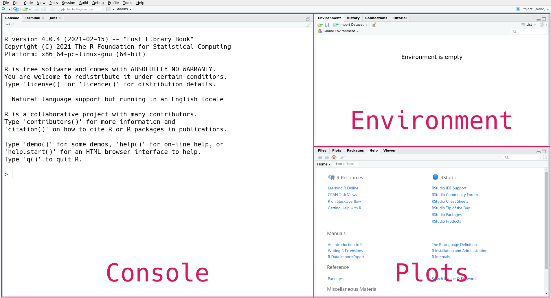
Don’t worry if the text in the panes isn’t exactly the same on your computer;
it depends on your operating system and versions of R and RStudio. The console
pane, on the left, is the main interface to R. If you type R code into the
console and press the Enter key on your keyboard, R will run your code and
return the result.
On the right are the environment pane and the plots pane. The environment pane shows data in your R workspace. The plots pane shows any plots you make, and also has tabs to browse your file system and to view R’s built-in help files. We’ll learn more about these gradually, but to get started we’ll focus on the console pane.
Let’s start by using R to do some arithmetic. In the console, you’ll see that
the cursor is on a line that begins with >, called the prompt. You can make
R compute the sum \(2 + 2\) by typing the code 2 + 2 after the prompt and then
pressing the Enter key. Your code and the result from R should look like
this:
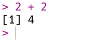
R always puts the result on a separate line (or lines) from your code. In this
case, the result begins with the tag [1], which is a hint from R that the
result is a vector and that this line starts with the element at position 1.
We’ll learn more about vectors in Section 2.1, and eventually learn
about other data types that are displayed differently. The result of the sum,
4, is displayed after the tag. In this reader, results from R will usually be
typeset in monospace and further prefixed with ## to indicate that they
aren’t code.
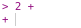
If you enter an incomplete expression, R will change the prompt to +, then
wait for you to type the rest of the expression and press the Enter key.
Here’s what it looks like if you only enter 2 +:
You can finish entering the expression, or you can cancel it by pressing the
Esc key (or Ctrl-c if you’re using R without RStudio). R can only tell an
expression is incomplete if it’s missing something, like the second operand in
2 +. So if you mean to enter 2 + 2 but accidentally enter 2, which is a
complete expression by itself, don’t expect R to read your mind and wait for
more input!
Try out some other arithmetic in the R console. Besides + for addition, the
other arithmetic operators are:
-for subtraction*for multiplication/for division%%for remainder division (modulo)^or**for exponentiation
You can combine these and use parentheses to make more complicated expressions, just as you would when writing a mathematical expression. When R computes a result, it follows the standard order of operations: parentheses, exponentiation, multiplication, division, addition, and finally subtraction. For example, to estimate the area of a circle with radius 3, you can write:
3.14 * 3^2## [1] 28.26You can write R expressions with any number of spaces (including none) around the operators and R will still compute the result. Nevertheless, putting spaces in your code makes it easier for you and others to read, so it’s good to make it a habit. Put spaces around most operators, after commas, and after keywords.
1.2.1 Variables
Since R is designed for mathematics and statistics, you might expect that it
provides a better appoximation for \(\pi\) than 3.14. R and most other
programming languages allow you to create named values, or variables. R
provides a built-in variable called pi for the value of \(\pi\). You can
display a variable’s value by entering its name in the console:
pi## [1] 3.141593You can also use variables in expressions. For instance, here’s a more precise expression for the area of a circle with radius 3:
pi * 3^2## [1] 28.27433You can define your own variables with the assignment operator = or <-. In
most circumstances these two operators are interchangeable. For clarity, it’s
best to choose one you like and use it consistently in all of your R code. In
this reader, we use = for assignment because this is the assignment operator
in most programming languages.
The main reason to use variables is to save results so that you can use them
on other expressions later. For example, to save the area of the circle in a
variable called area, we can write:
area = pi * 3^2In R, variable names can contain any combination of letters, numbers, dots .,
and underscores _, but must always start with a letter or a dot. Spaces and
other symbols are not allowed in variable names.
Now we can use the area variable anywhere we want the computed area. Notice
that when you assign a result to a variable, R doesn’t automatically display
that result. If you want to see the result as well, you have to enter the
variable’s name as a separate expression:
area## [1] 28.27433Another reason to use variables is to make an expression more general. For
instance, you might want to compute the area of several circles with different
radii. Then the expression pi * 3^2 is too specific. You can rewrite it as
pi * r^2, and then assign a value to the variable r just before you compute
the area. Here’s the code to compute and display the area of a circle with
radius 1 this way:
r = 1
area = pi * r^2
area
## [1] 3.141593Now if you want to compute the area for a different radius, all you have to do
is change r and run the code again (R will not change area until you do
this). Writing code that’s general enough to reuse across multiple problems can
be a big time-saver in the long run. Later on, we’ll see ways to make this code
even easier to reuse.
1.2.2 Strings
R treats anything inside single or double quotes as literal text rather than as an expression to evaluate. In programming jargon, a piece of literal text is called a string. You can use whichever kind of quotes you prefer, but the quote at the beginning of the string must match the quote at the end.
'Hi'## [1] "Hi""Hello!"## [1] "Hello!"Numbers and strings are not the same thing, so for example R considers 1
different from "1". As a result, you can’t use strings with most of R’s
arithmetic operators. For instance, this code causes an error:
"1" + 3## Error in "1" + 3: non-numeric argument to binary operatorThe error message notes that + is not defined for non-numeric values.
1.2.3 Comparisons
Besides arithmetic, you can also use R to compare values. The comparison operators are:
<for “less than”>for “greater than”<=for “less than or equal to”>=for “greater than or equal to”==for “equal to”!=for “not equal to”
The “equal to” operator uses two equal signs so that R can distinguish it from
=, the assignment operator.
Let’s look at a few examples:
1.5 < 3## [1] TRUE"a" > "b"## [1] FALSEpi == 3.14## [1] FALSE"hi" == 'hi'## [1] TRUEWhen you make a comparison, R returns a logical value, TRUE or FALSE, to
indicate the result. Logical values are not the same as strings, so they are
not quoted.
Logical values are values, so you can use them in other computations. For example:
TRUE## [1] TRUETRUE == FALSE## [1] FALSESection 2.4.5 describes more ways to use and combine logical values.
Beware that the equality operators don’t always return FALSE when you compare
two different types of data:
"1" == 1## [1] TRUE"TRUE" <= TRUE## [1] TRUE"FALSE" <= TRUE## [1] TRUESection 2.2.2 explains why this happens, and Appendix 5.1 explains several other ways to compare values.
1.2.4 Calling Functions
Most of R’s features are provided through functions, pieces of reusable code. You can think of a function as a machine that takes some inputs and uses them to produce some output. In programming jargon, the inputs to a function are called arguments, the output is called the return value, and when we use a function, we say we’re calling the function.
To call a function, write its name followed by parentheses. Put any arguments
to the function inside the parentheses. For example, in R, the sine function is
named sin (there are also cos and tan). So we can compute the sine of
\(\pi / 4\) with this code:
sin(pi / 4)## [1] 0.7071068There are many functions that accept more than one argument. For instance, the
sum function accepts any number of arguments and adds them all together. When
you call a function with multiple arguments, separate the arguments with
commas. So another way to compute \(2 + 2\) in R is:
sum(2, 2)## [1] 4When you call a function, R assigns each argument to a parameter. Parameters
are special variables that represent the inputs to a function and only exist
while that function runs. For example, the log function, which computes a
logarithm, has parameters x and base for the operand and base of the
logaritm, respectively. The next section, Section 1.3, explains
how to look up the parameters for a function.
By default, R assigns arguments to parameters based on their order. The first argument is assigned to the function’s first parameter, the second to the second, and so on. So we can compute the logarithm of 64, base 2, with this code:
log(64, 2)## [1] 6The argument 64 is assigned to the parameter x, and the argument 2 is
assigned to the parameter base. You can also assign arguments to parameters
by name with = (not <-), overriding their positions. So some other ways we
could write the call above are:
log(64, base = 2)## [1] 6log(x = 64, base = 2)## [1] 6log(base = 2, x = 64)## [1] 6log(base = 2, 64)## [1] 6All of these are equivalent. When you write code, choose whatever seems the clearest to you. Leaving parameter names out of calls saves typing, but including some or all of them can make the code easier to understand.
Parameters are not regular variables, and only exist while their associated function runs. You can’t set them before a call, nor can you access them after a call. So this code causes an error:
x = 64
log(base = 2)
## Error in eval(expr, envir, enclos): argument "x" is missing, with no defaultIn the error message, R says that we forgot to assign an argument to the
parameter x. We can keep the variable x and correct the call by making x
an argument (for the parameter x):
log(x, base = 2)## [1] 6Or, written more explicitly:
log(x = x, base = 2)## [1] 6In summary, variables and parameters are distinct, even if they happen to have
the same name. The variable x is not the same thing as the parameter x.
1.3 Getting Help
Learning and using a language is hard, so it’s important to know how to get
help. The first place to look for help is R’s built-in documentation. In the
console, you can access a specific help page by name with ? followed by the
name of the page.
There are help pages for all of R’s built-in functions, usually with the same
name as the function itself. So the code to open the help page for the log
function is:
?logFor functions, help pages usually include a brief description, a list of parameters, a description of the return value, and some examples.
There are also help pages for other topics, such as built-in mathematical
constants (such as ?pi), data sets (such as ?iris), and operators. To look
up the help page for an operator, put the operator’s name in single or double
quotes. For example, this code opens the help page for the arithmetic
operators:
?"+"It’s always okay to put quotes around the name of the page when you use ?,
but they’re only required if it contains non-alphabetic characters. So ?sqrt,
?'sqrt', and ?"sqrt" all open the documentation for sqrt, the square root
function.
Sometimes you might not know the name of the help page you want to look up. You
can do a general search of R’s help pages with ?? followed by a string of
search terms. For example, to get a list of all help pages related to linear
models:
??"linear model"This search function doesn’t always work well, and it’s often more efficient to use an online search engine. When you search for help with R online, include “R” as a search term. Alternatively, you can use RSeek, which restricts the search to a selection of R-related websites.
1.3.1 When Something Goes Wrong
As a programmer, sooner or later you’ll run some code and get an error message or result you didn’t expect. Don’t panic! Even experienced programmers make mistakes regularly, so learning how to diagnose and fix problems is vital.
Try going through these steps:
- If R returned a warning or error message, read it! If you’re not sure what the message means, try searching for it online.
- Check your code for typographical errors, including incorrect capitalization and missing or extra commas, quotes, and parentheses.
- Test your code one line at a time, starting from the beginning. After each line that assigns a variable, check that the value of the variable is what you expect. Try to determine the exact line where the problem originates (which may differ from the line that emits an error!).
If none of these steps help, try asking online. Stack Overflow is a popular question and answer website for programmers. Before posting, make sure to read about how to ask a good question.
1.4 File Systems
Most of the time, you won’t just write code directly into the R console. Reproducibility and reusability are important benefits of R over point-and-click software, and in order to realize these, you have to save your code to your computer’s hard drive. Let’s start by reviewing how files on a computer work. You’ll need to understand that before you can save your code, and it will also be important later on for loading data sets.
Your computer’s file system is a collection of files (chunks of data) and directories (or “folders”) that organize those files. For instance, the file system on a computer shared by Ada and Charles, two pioneers of computing, might look like this:
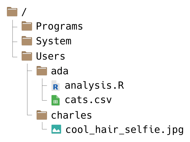
Don’t worry if your file system looks a bit different from the picture.
File systems have a tree-like structure, with a top-level directory called the
root directory. On Ada and Charles’ computer, the root is called /, which
is also what it’s called on all macOS and Linux computers. On Windows, the root
is usually called C:/, but sometimes other letters, like D:/, are also used
depending on the computer’s hardware.
A path is a list of directories that leads to a specific file or directory on
a file system (imagine giving directons to someone as they walk through the
file system). We use forward slashes / to separate the directories in a path,
rather than commas or spaces. The root directory includes a forward slash as
part of its name, and doesn’t need an extra one.
For example, suppose Ada wants to write a path to the file cats.csv. She can
write the path like this:
/Users/ada/cats.csvYou can read this path from left-to-right as, “Starting from the root
directory, go to the Users directory, then from there go to the ada
directory, and from there go to the file cats.csv.” Alternatively, you can
read the path from right-to-left as, “The file cats.csv inside of the ada
directory, which is inside of the Users directory, which is in the root
directory.”
As another example, suppose Charles wants a path to the Programs directory.
He can write:
/Programs/The / at the end of this path is reminder that Programs is a directory, not
a file. Charles could also write the path like this:
/ProgramsThis is still correct, but it’s not as obvious that Programs is a directory.
In other words, when a path leads to a directory, including a trailing slash
is optional, but makes the meaning of the path clearer. Paths that lead to
files never have a trailing slash.
On Windows computers, paths are usually written with backslashes \ to
separate directories instead of forward slashes. Fortunately, R uses forward
slashes / for all paths, regardless of the operating system. So when you’re
working in R, use forward slashes and don’t worry about the operating system.
This is especially convenient when you want to share code with someone that
uses a different operating system than you.
1.4.1 Absolute & Relative Paths
A path that starts from the root directory, like all of the ones we’ve seen so far, is called an absolute path. The path is “absolute” because it unambiguously describes where a file or directory is located. The downside is that absolute paths usually don’t work well if you share your code.
For example, suppose Ada uses the path /Programs/ada/cats.csv to load the
cats.csv file in her code. If she shares her code with another pioneer of
computing, say Gladys, who also has a copy of cats.csv, it might
not work. Even though Gladys has the file, she might not have it in a directory
called ada, and might not even have a directory called ada on her computer.
Because Ada used an absolute path, her code works on her own computer, but
isn’t portable to others.
On the other hand, a relative path is one that doesn’t start from the root directory. The path is “relative” to an unspecified starting point, which usually depends on the context.
For instance, suppose Ada’s code is saved in the file analysis.R (more about
.R files in Section 1.4.2), which is in the same directory as
cats.csv on her computer. Then instead of an absolute path, she can use a
relative path in her code:
cats.csvThe context is the location of analysis.R, the file that contains the code.
In other words, the starting point on Ada’s computer is the ada directory. On
other computers, the starting point will be different, depending on where the
code is stored.
Now suppose Ada sends her corrected code in analysis.R to Gladys, and tells
Gladys to put it in the same directory as cats.csv. Since the path cats.csv
is relative, the code will still work on Gladys’ computer, as long as the two
files are in the same directory. The name of that directory and its location in
the file system don’t matter, and don’t have to be the same as on Ada’s
computer. Gladys can put the files in a directory /Users/gladys/from_ada/ and
the path (and code) will still work.
Relative paths can include directories. For example, suppose that Charles wants
to write a relative path from the Users directory to a cool selfie he took.
Then he can write:
charles/cool_hair_selfie.jpgYou can read this path as, “Starting from wherever you are, go to the charles
directory, and from there go to the cool_hair_selfie.jpg file.” In other
words, the relative path depends on the context of the code or program that
uses it.
When use you paths in R code, they should almost always be relative paths. This ensures that the code is portable to other computers, which is an important aspect of reproducibility. Another benefit is that relative paths tend to be shorter, making your code easier to read (and write).
When you write paths, there are three shortcuts you can use. These are most useful in relative paths, but also work in absolute paths:
.means the current directory...means the directory above the current directory.~means the home directory. Each user has their own home directory, whose location depends on the operating system and their username. Home directories are typically found insideC:/Users/on Windows,/Users/on macOS, and/home/on Linux.
As an example, suppose Ada wants to write a (relative) path from the ada
directory to Charles’ cool selfie. Using these shorcuts, she can write:
../charles/cool_hair_selfie.jpgRead this as, “Starting from wherever you are, go up one directory, then go to
the charles directory, and then go to the cool_hair_selfie.jpg file.” Since
/Users/ada is Ada’s home directory, she could also write the path as:
~/../charles/cool_hair_selfie.jpgThis path has the same effect, but the meaning is slightly different. You can
read it as “Starting from your home directory, go up one directory, then go to
the charles directory, and then go to the cool_hair_selfie.jpg file.”
The .. and ~ shortcut are frequently used and worth remembering. The .
shortcut is included here in case you see it in someone else’s code. Since it
means the current directory, a path like ./cats.csv is identical to
cats.csv, and the latter is preferable for being simpler. There are a few
specific situations where . is necessary, but they fall outside the scope of
this text.
1.4.2 R Scripts
Now that you know how file systems and paths work, you’re ready to learn how to
save your R code to a file. R code is usually saved into an R script
(extension .R) or an R Markdown file (extension .Rmd). R scripts are
slightly simpler, so let’s focus on those.
In RStudio, you can create a new R script with this menu option:
File -> New File -> R ScriptThis will open a new pane in RStudio, like this:
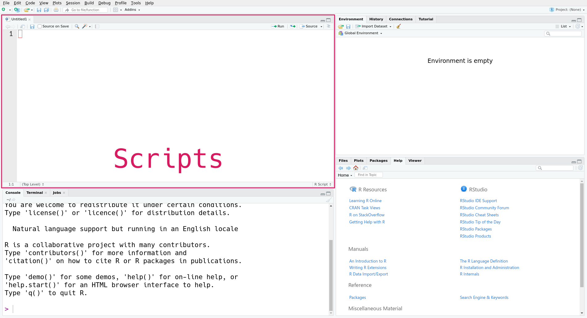
The new pane is the scripts pane, which displays all of the R scripts you’re editing. Each script appears in a separate tab. In the screenshot, only one script, the new script, is open.
Editing a script is similar to editing any other text document. You can write, delete, copy, cut, and paste text. You can also save the file to your computer’s file system. When you do, pay attention to where you save the file, as you might need it later.
The contents of an R script should be R code. Anything else you want to write
in the script (notes, documentation, etc.) should be in a comment. In R,
comments begin with # and extend to the end of the line:
# This is a comment.R will ignore comments when you run your code.
When you start a new project, it’s a good idea to create a specific directory for all of the project’s files. If you’re using R, you should also create one or more R scripts in that directory. As you work, write your code directly into a script. Arrange your code in the order of the steps to solve the problem, even if you write some parts before others. Comment out or delete any lines of code that you try but ultimately decide you don’t need. Make sure to save the file periodically so that you don’t lose your work. Following these guidelines will help you stay organized and make it easier to share your code with others later.
While editing, you can run the current line in the R console by pressing
Ctrl+Enter on Windows and Linux, or Cmd+Enter on macOS. This way you
can test and correct your code as you write it.
If you want, you can instead run (or source) the entire R script, by calling
the source function with the path to the script as an argument. This is also
what the “Source on Save” check box refers to in RStudio. The code runs in
order, only stopping if an error occurs.
For instance, if you save the script as my_cool_script.R, then you can run
source("my_cool_script.R") in the console to run the entire script (pay
attention to the path—it may be different on your computer).
R Markdown files are an alternative format for storing R code. They provide a richer set of formatting options, and are usually a better choice than R scripts if you’re writing a report that contains code. You can learn more about R Markdown files here.
1.4.3 The Working Directory
Section 1.4.1 explained that relative paths have a starting point that depends on the context where the path is used. We can make that idea more concrete for R. The working directory is the starting point R uses for relative paths. Think of the working directory as the directory R is currently “at” or watching.
The function getwd returns the absolute path for the current working
directory, as a string. It doesn’t require any arguments:
getwd()## [1] "/home/nick/workshop/datalab/workshops/r_basics"On your computer, the output from getwd will likely be different. This is a
very useful function for getting your bearings when you write relative paths.
If you write a relative path and it doesn’t work as expected, the first thing
to do is check the working directory.
The related setwd function changes the working directory. It takes one
argument: a path to the new working directory. Here’s an example:
setwd("..")

# Now check the working directory.
getwd()
Generally, you should avoid using calls to setwd in your R scripts and R
Markdown files. Calling setwd makes your code more difficult to understand,
and can always be avoided by using appropriate relative paths. If you call
setwd with an absolute path, it also makes your code less portable to other
computers. It’s fine to use setwd interactively (in the R console), but avoid
making your saved code dependent on it.
Another function that’s useful for dealing with the working directory and file
system is list.files. The list.files function returns the names of all of
the files and directories inside of a directory. It accepts a path to a
directory as an argument, or assumes the working directory if you don’t pass a
path. For instance:
# List files and directories in /home/.
list.files("/home/")
## [1] "lost+found" "nick"# List files and directories in the working directory.
list.files()## [1] "_bookdown_files" "_bookdown.yml"
## [3] "_main.rds" "01_getting-started.Rmd"
## [5] "02_data-structures.Rmd" "03_exploring-data_files"
## [7] "03_exploring-data.Rmd" "04_automating-tasks.Rmd"
## [9] "05_appendix.Rmd" "97_where-to-learn-more.Rmd"
## [11] "98_acknowledgements.Rmd" "99_assessment.Rmd"
## [13] "assessment" "data"
## [15] "docs" "graphviz"
## [17] "img" "index.md"
## [19] "index.Rmd" "knit.R"
## [21] "LICENSE" "makefile"
## [23] "notes" "R"
## [25] "raw" "README.md"
## [27] "rendere73e1982629f.rds" "renv"
## [29] "renv.lock"As usual, since you have a different computer, you’re likely to see different
output if you run this code. If you call list.files with an invalid path or
an empty directory, the output is character(0):
list.files("/this/path/is/fake/")## character(0)Later on, we’ll learn about what character(0) means more generally.
1.5 Reading Files
Analyzing data sets is one of the most common things to do in R. The first step is to get R to read your data. Data sets come in a variety of file formats, and you need to identify the format in order to tell R how to read the data.
Most of the time, you can guess the format of a file by looking at its
extension, the characters (usually three) after the last dot . in the
filename. For example, the extension .jpg or .jpeg indicates a JPEG image
file. Some operating systems hide extensions by default, but you can find
instructions to change this setting online by searching for “show file
extensions” and your operating system’s name. The extension is just part of the
file’s name, so it should be taken as a hint about the file’s format rather
than a guarantee.
R has built-in functions for reading a variety of formats. The R community also provides packages, shareable and reusable pieces of code, to read even more formats. You’ll learn more about packages later, in Section 3.2. For now, let’s focus on data sets that can be read with R’s built-in functions.
Here are several formats that are frequently used to distribute data, along with the name of a built-in function or contributed package that can read the format:
| Name | Extension | Function or Package | Tabular? | Text? |
|---|---|---|---|---|
| Comma-separated Values | .csv |
read.csv |
Yes | Yes |
| Tab-separated Values | .tsv |
read.delim |
Yes | Yes |
| Fixed-width File | .fwf |
read.fwf |
Yes | Yes |
| Microsoft Excel | .xlsx |
readr package | Yes | No |
| Microsoft Excel 1993-2007 | .xls |
readr package | Yes | No |
| Apache Arrow | .feather |
arrow package | Yes | No |
| R Data | .rds |
readRDS |
Sometimes | No |
| R Data | .rda |
load |
Sometimes | No |
| Plaintext | .txt |
readLines |
Sometimes | Yes |
| Extensible Markup Language | .xml |
xml2 package | No | Yes |
| JavaScript Object Notation | .json |
jsonlite package | No | Yes |
A tabular data set is one that’s structured as a table, with rows and columns. We’ll focus on tabular data sets for most of this reader, since they’re easier to get started with. Here’s an example of a tabular data set:
| Fruit | Quantity | Price |
|---|---|---|
| apple | 32 | 1.49 |
| banana | 541 | 0.79 |
| pear | 10 | 1.99 |
A text file is one that contains human-readable lines of text. You can check this by opening the file with a text editor such as Microsoft Notepad or macOS TextEdit. Many file formats use text in order to make the format easier to work with.
For instance, a comma-separated values (CSV) file records a tabular data using one line per row, with commas separating columns. If you store the table above in a CSV file and open the file in a text editor, here’s what you’ll see:
Fruit,Quantity,Price
apple,32,1.49
banana,541,0.79
pear,10,1.99
A binary file is one that’s not human-readable. You can’t just read off the data if you open a binary file in a text editor, but they have a number of other advantages. Compared to text files, binary files are often faster to read and take up less storage space (bytes).
As an example, R’s built-in binary format is called RDS (which may stand for
“R data serialized”). RDS files are extremely useful for backing up work, since
they can store any kind of R object, even ones that are not tabular. You can
learn more about how to create an RDS file on the ?saveRDS help page, and how
to read one on the ?readRDS help page.
1.5.1 Hello, Data!
Let’s read our first data set! Over the next few sections, we’re going to
explore data from the U.S. Bureau of Labor Statistics about median employee
earnings. The data set was prepared as part of the Tidy Tuesday R community
project. You can find more details about the data set here, and you can
download the data set here (you may need to choose File -> Save As... in your browser’s menu).
The data set is a file called earn.csv, which suggests it’s a CSV file. In
this case, the extension is correct, so we can read the file into R with the
built-in read.csv function. The first argument is the path to where you saved
the file, which may be different on your computer. The read.csv function
returns the data set, but R won’t keep the data in memory unless we assign the
returned result to a variable:
earn = read.csv("data/earn.csv")The variable name earn here is arbitrary; you can choose something different
if you want. However, in general, it’s a good habit to choose variable names
that describe the contents of the variable somehow.
If you tried running the line of code above and got an error message, pay attention to what the error message says, and remember the strategies to get help in Section 1.3. The most common mistake when reading a file is incorrectly specifying the path, so first check that you got the path right.
If you ran the line of code and there was no error message, congratulations, you’ve read your first data set into R!
1.6 Data Frames
Now that we’ve loaded the data, let’s take a look at it. When you’re working
with a new data set, it’s usually not a good idea to print it out directly (by
typing earn, in this case) until you know how big it is. Big data sets can
take a long time to print, and the output can be difficult to read.
Instead, you can use the head function to print only the beginning, or
head, of a data set. Let’s take a peek:
head(earn)## sex race ethnic_origin age year quarter n_persons
## 1 Both Sexes All Races All Origins 16 years and over 2010 1 96821000
## 2 Both Sexes All Races All Origins 16 years and over 2010 2 99798000
## 3 Both Sexes All Races All Origins 16 years and over 2010 3 101385000
## 4 Both Sexes All Races All Origins 16 years and over 2010 4 100120000
## 5 Both Sexes All Races All Origins 16 years and over 2011 1 98329000
## 6 Both Sexes All Races All Origins 16 years and over 2011 2 100593000
## median_weekly_earn
## 1 754
## 2 740
## 3 740
## 4 752
## 5 755
## 6 753This data set is tabular—as you might have already guessed, since it came
from a CSV file. In R, it’s represented by a data frame, a table with rows
and columns. R uses data frames to represent most (but not all) kinds of
tabular data. The read.csv function, which we used to read this data, always
returns a data frame.
For a data frame, the head function only prints the first six rows. If there
are lots of columns or the columns are wide, as is the case here, R wraps the
output across lines.
When you first read an object into R, you might not know whether it’s a data
frame. One way to check is visually, by printing it, as we just did. A better
way to check is with the class function, which returns information about what
an object is. For a data frame, the result will always contain data.frame:
class(earn)## [1] "data.frame"We’ll learn more about classes in Section 2.2, but for now you can use this function to identify data frames.
By counting the columns in the output from head(earn), we can see that this
data set has eight columns. A more convenient way to check the number of
columns in a data set is with the ncol function:
ncol(earn)## [1] 8The similarly-named nrow function returns the number of rows:
nrow(earn)## [1] 4224Alternatively, you can get both numbers at the same time with the dim (short
for “dimensions”) function.
Since the columns have names, we might also want to get just these. You can do
that with the names or colnames functions. Both return the same result:
names(earn)## [1] "sex" "race" "ethnic_origin"
## [4] "age" "year" "quarter"
## [7] "n_persons" "median_weekly_earn"colnames(earn)## [1] "sex" "race" "ethnic_origin"
## [4] "age" "year" "quarter"
## [7] "n_persons" "median_weekly_earn"If the rows have names, you can get those with the rownames function. For
this particular data set, the rows don’t have names.
1.6.1 Summarizing Data
An efficient way to get a sense of what’s actually in a data set is to have R
compute summary information. This works especially well for data frames, but
also applies to other data. R provides two different functions to get
summaries: str and summary.
The str function returns a structural summary of an object. This kind of
summary tells us about the structure of the data—the number of rows, the
number and names of columns, what kind of data is in each column, and some
sample values. Here’s the structural summary for the earnings data:
str(earn)## 'data.frame': 4224 obs. of 8 variables:
## $ sex : chr "Both Sexes" "Both Sexes" "Both Sexes" "Both Sexes" ...
## $ race : chr "All Races" "All Races" "All Races" "All Races" ...
## $ ethnic_origin : chr "All Origins" "All Origins" "All Origins" "All Origins" ...
## $ age : chr "16 years and over" "16 years and over" "16 years and over" "16 years and over" ...
## $ year : int 2010 2010 2010 2010 2011 2011 2011 2011 2012 2012 ...
## $ quarter : int 1 2 3 4 1 2 3 4 1 2 ...
## $ n_persons : int 96821000 99798000 101385000 100120000 98329000 100593000 101447000 101458000 100830000 102769000 ...
## $ median_weekly_earn: int 754 740 740 752 755 753 753 764 769 771 ...This summary lists information about each column, and includes most of what we
found earlier by using several different functions separately. The summary uses
chr to indicate columns of text (“characters”) and int to indicate columns
of integers.
In contrast to str, the summary function returns a statistical summary of
an object. This summary includes summary statistics for each column, choosing
appropriate statistics based on the kind of data in the column. For numbers,
this is generally the mean, median, and quantiles. For categories, this is the
frequencies. Other kinds of statistics are shown for other kinds of data.
Here’s the statistical summary for the earnings data:
summary(earn)## sex race ethnic_origin age
## Length:4224 Length:4224 Length:4224 Length:4224
## Class :character Class :character Class :character Class :character
## Mode :character Mode :character Mode :character Mode :character
##
##
##
## year quarter n_persons median_weekly_earn
## Min. :2010 Min. :1.00 Min. : 103000 Min. : 318.0
## 1st Qu.:2012 1st Qu.:1.75 1st Qu.: 2614000 1st Qu.: 605.0
## Median :2015 Median :2.50 Median : 7441000 Median : 755.0
## Mean :2015 Mean :2.50 Mean : 16268338 Mean : 762.2
## 3rd Qu.:2018 3rd Qu.:3.25 3rd Qu.: 17555250 3rd Qu.: 911.0
## Max. :2020 Max. :4.00 Max. :118358000 Max. :1709.01.6.2 Selecting Columns
You can select an individual column from a data frame by name with $, the
dollar sign operator. The syntax is:
VARIABLE$COLUMN_NAMEFor instance, for the earnings data, earn$age selects
the age column, and earn$n_persons selects the n_persons column. So one
way to compute the mean of the n_persons column is:
mean(earn$n_persons)## [1] 16268338Similarly, to compute the range of the year column:
range(earn$year)## [1] 2010 2020You can also use the dollar sign operator to assign values to columns. For
instance, to assign 0 to the entire quarter column:
earn$quarter = 0Be careful when you do this, as there is no undo. Fortunately, we haven’t
applied any transformations to the earnings data yet, so we can reset the
earn variable back to what it was by reloading the data set:
earn = read.csv("data/earn.csv")In Section 2.4, we’ll learn how to select rows and individual elements from a data frame, as well as other ways to select columns.
1.7 Exercises
1.7.1 Exercise
In a string, an escape sequence or escape code consists of a backslash followed by one or more characters. Escape sequences make it possible to:
- Write quotes or backslashes within a string
- Write characters that don’t appear on your keyboard (for example, characters in a foreign language)
For example, the escape sequence \n corresponds to the newline character.
There’s a complete list of escape sequences for R in the ?Quotes help file.
Other programming languages also use escape sequences, and many of them are the
same as in R.
- Assign a string that contains a newline to the variable
newline. Then make R display the value of the variable by enteringnewlineat the R prompt. - The
messagefunction prints output to the R console, so it’s one way you can make your R code report information as it runs. Use themessagefunction to printnewline. - How does the output from part 1 compare to the output from part 2? Why do you think they differ?
1.7.2 Exercise
Choose a directory on your computer that you’re familiar with, such as one you created. Determine the path to the directory, then use
list.filesto display its contents. Do the files displayed match what you see in your system’s file browser?What does the
all.filesparameter oflist.filesdo? Give an example.
1.7.3 Exercise
The read.table function is another function for reading tabular data. Take a
look at the help file for read.table. Recall that read.csv reads tabular
data where the values are separated by commas, and read.delim reads tabular
data where the values are separated by tabs.
- What value-separator does
read.tableexpect by default? - Is it possible to use
read.tableto read a CSV? Explain. If your answer is yes, show how to useread.tableto load the employee earnings data from Section 1.5.1.