2 Tidy & Relational Data

This chapter is part 2 (of 2) of Cleaning & Reshaping Data, a workshop series about how to prepare data for analysis. The major topics of this chapter are how to reshape datasets with pivots and how to combine related datasets with joins

Learning Objectives

After completing this session, learners should be able to:

Explain what it means for data to be tidy
Use the tidyr package to reshape data
Explain what a relational dataset is
Use the dplyr package to join data based on common columns
Describe the different types of joins
Identify which types of joins to use when faced with a relational dataset

2.1 Tidy Datasets

The structure of a dataset—its shape and organization—has enormous influence on how difficult it will be to analyze, so making structural changes is an important part of the cleaning process. Researchers conventionally arrange tabular datasets so that each row contains a single observation or case, and each column contains a single kind of measurement or identifier, called a feature.

In 2014, Hadley Wickham refined and formalized the conventions for tabular datasets by introducing the concept of tidy datasets, which have a specific structure. Paraphrasing Wickham, the rules for a tidy dataset are:

Every column is a single feature.

Every row is a single observation.

Every cell is a single value.

These rules ensure that all of the values in a dataset are visually organized and are easy to access with indexing operations. They’re also specific enough to make tidiness a convenient standard for functions that operate on tabular datasets. In fact, the Tidyverse packages (see Section 1.1) are designed from the ground up for working with tidy datasets. Tidy datesets have also been adopted as a standard in other software, including various packages for Python and Julia.

This section explains how to reshape tabular datasets into tidy datasets. While reshaping can seem tricky at first, making sure your dataset has the right structure before you begin analysis saves time and frustration in the long run.

2.1.1 The tidyr Package

The tidyr package provides functions to reshape tabular datasets. It also provides examples of tidy and untidy datasets. Like most Tidyverse packages, it comes with detailed documentation and a cheatsheet.

As usual, install the package if you haven’t already, and then load it:

# install.packages("tidyr")
library(tidyr)

Let’s start with an example of a tidy dataset. The table1 dataset in the package records the number of tuberculosis cases across several different countries and years:

table1

## # A tibble: 6 × 4
##   country      year  cases population
##   <chr>       <dbl>  <dbl>      <dbl>
## 1 Afghanistan  1999    745   19987071
## 2 Afghanistan  2000   2666   20595360
## 3 Brazil       1999  37737  172006362
## 4 Brazil       2000  80488  174504898
## 5 China        1999 212258 1272915272
## 6 China        2000 213766 1280428583

Each of the four columns contains a single kind of measurement or identifier, so the dataset satifies tidy rule 1. The measurements were taken at the country-year level, and each row contains data for one country-year pair, so the dataset also satisfies tidy rule 2. Each cell in the data frame only contains one value, so the dataset also satisfies tidy rule 3.

The same data are recorded in table2, table3, and the pair table4a with table4b, but these are all untidy datasets. For example, table2 breaks rule 1 because the column count contains two different kinds of measurements—case counts and population counts:

table2

## # A tibble: 12 × 4
##    country      year type            count
##    <chr>       <dbl> <chr>           <dbl>
##  1 Afghanistan  1999 cases             745
##  2 Afghanistan  1999 population   19987071
##  3 Afghanistan  2000 cases            2666
##  4 Afghanistan  2000 population   20595360
##  5 Brazil       1999 cases           37737
##  6 Brazil       1999 population  172006362
##  7 Brazil       2000 cases           80488
##  8 Brazil       2000 population  174504898
##  9 China        1999 cases          212258
## 10 China        1999 population 1272915272
## 11 China        2000 cases          213766
## 12 China        2000 population 1280428583

When considering whether you should reshape a dataset, think about what the features are and what the observations are. These depend on the dataset itself, but also on what kinds of analyses you want to do. Datasets sometimes have closely related features or multiple (nested) levels of observation. The tidyr documentation includes a detailed article on how to reason about reshaping datasets.

If you do decide to reshape a dataset, then you should also think about what role each feature serves:

Identifiers are labels that distinguish observations from one another. They are often but not always categorical. Examples include names or identification numbers, treatment groups, and dates or times. In the tuberculosis data set, the country and year columns are identifiers.
Measurements are the values collected for each observation and typically the values of research interest. For the tuberculosis data set, the cases and population columns are measurements.

Having a clear understanding of which features are identifiers and which are measurements makes it easier to use the tidyr functions.

2.1.2 Rows into Columns

Tidy data rule 1 is that each column must be a single feature. The table2 dataset breaks this rule:

table2

## # A tibble: 12 × 4
##    country      year type            count
##    <chr>       <dbl> <chr>           <dbl>
##  1 Afghanistan  1999 cases             745
##  2 Afghanistan  1999 population   19987071
##  3 Afghanistan  2000 cases            2666
##  4 Afghanistan  2000 population   20595360
##  5 Brazil       1999 cases           37737
##  6 Brazil       1999 population  172006362
##  7 Brazil       2000 cases           80488
##  8 Brazil       2000 population  174504898
##  9 China        1999 cases          212258
## 10 China        1999 population 1272915272
## 11 China        2000 cases          213766
## 12 China        2000 population 1280428583

To make the dataset tidy, the measurements in the count column need to be separated into two separate columns, cases and population, based on the categories in the type column.

You can use the pivot_wider function to pivot the single count column into two columns according to the type column. This makes the dataset wider, hence the name pivot_wider.

The function’s first parameter is the dataset to pivot. Other important parameters are:

values_from – The column(s) to pivot.
names_from – The column that contains names for the new columns.
id_cols – The identifier columns, which are not pivoted. This defaults to all columns except those in values_from and names_from.

Here’s how to use the function to make table2 tidy:

pivot_wider(table2, values_from = count, names_from = type)

## # A tibble: 6 × 4
##   country      year  cases population
##   <chr>       <dbl>  <dbl>      <dbl>
## 1 Afghanistan  1999    745   19987071
## 2 Afghanistan  2000   2666   20595360
## 3 Brazil       1999  37737  172006362
## 4 Brazil       2000  80488  174504898
## 5 China        1999 212258 1272915272
## 6 China        2000 213766 1280428583

The function automatically removes values from the country and year columns as needed to maintain their original correspondence with the pivoted values.

2.1.3 Columns into Rows

Tidy data rule 2 is that every row must be a single observation. The table4a and table4b datasets break this rule because each row in each dataset contains measurements for two different years:

table4a

## # A tibble: 3 × 3
##   country     `1999` `2000`
##   <chr>        <dbl>  <dbl>
## 1 Afghanistan    745   2666
## 2 Brazil       37737  80488
## 3 China       212258 213766

table4b

## # A tibble: 3 × 3
##   country         `1999`     `2000`
##   <chr>            <dbl>      <dbl>
## 1 Afghanistan   19987071   20595360
## 2 Brazil       172006362  174504898
## 3 China       1272915272 1280428583

The tuberculosis case counts are in table4a. The population counts are in table4b. Neither is tidy.

To make the table4a dataset tidy, the 1999 and 2000 columns need to be pivoted into two new columns: one for the measurements (the counts) and one for the identifiers (the years). It might help to visualize this as stacking the two separate columns 1999 and 2000 together, one on top of the other, and then adding a second column with the appropriate years. The same process makes table4b tidy.

You can use the pivot_longer function to pivot the two columns 1999 and 2000 into a column of counts and a column of years. This makes the dataset longer, hence the name pivot_longer.

Again the function’s first parameter is the dataset to pivot. Other important parameters are:

cols – The columns to pivot.
values_to – Name(s) for the new measurement column(s)
names_to – Name(s) for the new identifier column(s)

Here’s how to use the function to make table4a tidy:

tidy4a = pivot_longer(table4a, -country, values_to = "cases",
  names_to = "year")
tidy4a

## # A tibble: 6 × 3
##   country     year   cases
##   <chr>       <chr>  <dbl>
## 1 Afghanistan 1999     745
## 2 Afghanistan 2000    2666
## 3 Brazil      1999   37737
## 4 Brazil      2000   80488
## 5 China       1999  212258
## 6 China       2000  213766

In this case, the cols parameter is set to all columns except the country column, because the country column does not need to be pivoted. The function automatically repeats values in the country column as needed to maintain its original correspondence with the pivoted values.

Here’s the same for table4b:

tidy4b = pivot_longer(table4b, -country, values_to = "population",
  names_to = "year")
tidy4b

## # A tibble: 6 × 3
##   country     year  population
##   <chr>       <chr>      <dbl>
## 1 Afghanistan 1999    19987071
## 2 Afghanistan 2000    20595360
## 3 Brazil      1999   172006362
## 4 Brazil      2000   174504898
## 5 China       1999  1272915272
## 6 China       2000  1280428583

Once the two datasets are tidy, you can join them with the merge function to reproduce table1:

merge(tidy4a, tidy4b)

##       country year  cases population
## 1 Afghanistan 1999    745   19987071
## 2 Afghanistan 2000   2666   20595360
## 3      Brazil 1999  37737  172006362
## 4      Brazil 2000  80488  174504898
## 5       China 1999 212258 1272915272
## 6       China 2000 213766 1280428583

2.1.4 Separating Values

Tidy data rule 3 says each value must have its own cell. The table3 dataset breaks this rule because the rate column contains two values per cell:

table3

## # A tibble: 6 × 3
##   country      year rate             
##   <chr>       <dbl> <chr>            
## 1 Afghanistan  1999 745/19987071     
## 2 Afghanistan  2000 2666/20595360    
## 3 Brazil       1999 37737/172006362  
## 4 Brazil       2000 80488/174504898  
## 5 China        1999 212258/1272915272
## 6 China        2000 213766/1280428583

The two values separated by / in the rate column are the tuberculosis case count and the population count.

To make this dataset tidy, the rate column needs to be split into two columns, cases and population. The values in the rate column are strings, so one way to do this is with the stringr package’s str_split_fixed function, described in Section 1.4.4:

library(stringr)

# Split the rate column into 2 columns.
cols = str_split_fixed(table3$rate, fixed("/"), 2)

# Remove the rate column and append the 2 new columns.
tidy3 = table3[-3]
tidy3$cases = as.numeric(cols[, 1])
tidy3$population = as.numeric(cols[, 2])
tidy3

## # A tibble: 6 × 4
##   country      year  cases population
##   <chr>       <dbl>  <dbl>      <dbl>
## 1 Afghanistan  1999    745   19987071
## 2 Afghanistan  2000   2666   20595360
## 3 Brazil       1999  37737  172006362
## 4 Brazil       2000  80488  174504898
## 5 China        1999 212258 1272915272
## 6 China        2000 213766 1280428583

Extracting values, converting to appropriate data types, and then combining everything back into a single data frame is an extremely common pattern in data science.

The tidyr package provides the separate function to streamline the steps taken above. The first parameter is the dataset, the second is the column to split, the third is the names of the new columns, and the fourth is the delimiter. The convert parameter controls whether the new columns are automatically converted to appropriate data types:

separate(table3, rate, c("cases", "population"), "/", convert = TRUE)

## # A tibble: 6 × 4
##   country      year  cases population
##   <chr>       <dbl>  <int>      <int>
## 1 Afghanistan  1999    745   19987071
## 2 Afghanistan  2000   2666   20595360
## 3 Brazil       1999  37737  172006362
## 4 Brazil       2000  80488  174504898
## 5 China        1999 212258 1272915272
## 6 China        2000 213766 1280428583

As of writing, the tidyr developers have deprecated the separate function in favor of several more specific functions (separate_wider_delim, separate_wider_position, and separate_wider_regex). These functions are still experimental, so we still recommend using the separate function in the short term.

2.1.5 Case Study: SMART Ridership

Sonoma-Marin Area Rail Transit (SMART) is a single-line passenger rail service between the San Francisco Bay and Santa Rosa. They publish data about monthly ridership in PDF and Excel format. In this case study, you’ll reshape and clean the dataset to prepare it for analysis.

To get started, download the [February 2024 report in Excel format][smart-jan24]. Pay attention to where you save the file—or move it to a directory just for files related to this case study—so that you can load it into R. If you want, you can use R’s download.file function to download the file rather than your browser.

The readxl package provides functions to read data from Excel files. Install the package if you don’t already have it installed, and then load it:

# install.packages("readxl")
library("readxl")

You can use the read_excel function to read a sheet from an Excel spreadsheet. Before doing so, it’s a good idea to manually inspect the spreadsheet in a spreadsheet program. The SMART dataset contains two tables in the first sheet, one for total monthly ridership and another for average weekday ridership (by month).

Let’s focus on the total monthly ridership table, which occupies cells B4 to H16. You can specify a range of cells when you call read_excel by setting the range parameter:

smart_path = "./data/SMART Ridership Web Posting_1.24.xlsx"
smart = read_excel(smart_path, range = "B4:I16")
smart

## # A tibble: 12 × 8
##    Month FY18   FY19   FY20  FY21   FY22  FY23  FY24
##    <chr> <chr> <dbl>  <dbl> <dbl>  <dbl> <dbl> <dbl>
##  1 Jul   -     63864 62851   9427 24627  43752 65779
##  2 Aug   54484 74384 65352   8703 25020  48278 72171
##  3 Sep   65019 62314 62974   8910 27967  49134 68506
##  4 Oct   57453 65492 57222   9851 26998. 59322 70807
##  5 Nov   56125 52774 64966   8145 26575  51383 65445
##  6 Dec   56425 51670 58199.  7414 24050  47606 66684
##  7 Jan   56527 57136 71974   6728 22710  46149 65990
##  8 Feb   54797 51130 71676   7412 26652  49724    NA
##  9 Mar   57312 58091 33624   9933 35291  53622    NA
## 10 Apr   56631 60256  4571  11908 34258  58551    NA
## 11 May   59428 64036  5308  13949 38655  65416    NA
## 12 Jun   61828 55700  8386  20469 41525  67162    NA

The loaded dataset needs to be cleaned. The FY18 column uses a hyphen to indicate missing data and has the wrong data type. The identifiers—months and years—are split between the row and column names and each row contains data from seven different years, so the dataset is also not tidy. In addition, the years are indicated in fiscal years (FY), which begin in July rather than January, so some of the years need to be adjusted.

You can correct the missing value in the FY18 column with indexing, and the type with the as.numeric function:

smart$FY18[smart$FY18 == "-"] = NA
smart$FY18 = as.numeric(smart$FY18)
head(smart)

## # A tibble: 6 × 8
##   Month  FY18  FY19   FY20  FY21   FY22  FY23  FY24
##   <chr> <dbl> <dbl>  <dbl> <dbl>  <dbl> <dbl> <dbl>
## 1 Jul      NA 63864 62851   9427 24627  43752 65779
## 2 Aug   54484 74384 65352   8703 25020  48278 72171
## 3 Sep   65019 62314 62974   8910 27967  49134 68506
## 4 Oct   57453 65492 57222   9851 26998. 59322 70807
## 5 Nov   56125 52774 64966   8145 26575  51383 65445
## 6 Dec   56425 51670 58199.  7414 24050  47606 66684

To make the dataset tidy, it needs to be reshaped so that the values in the various fiscal year columns are all in one column. In other words, the dataset needs to be pivoted longer (Section 2.1.3). The result of the pivot will be easier to understand if you rename the columns as their years first. Here’s one way to do that:

names(smart)[-1] = 2018:2024
head(smart)

## # A tibble: 6 × 8
##   Month `2018` `2019` `2020` `2021` `2022` `2023` `2024`
##   <chr>  <dbl>  <dbl>  <dbl>  <dbl>  <dbl>  <dbl>  <dbl>
## 1 Jul       NA  63864 62851    9427 24627   43752  65779
## 2 Aug    54484  74384 65352    8703 25020   48278  72171
## 3 Sep    65019  62314 62974    8910 27967   49134  68506
## 4 Oct    57453  65492 57222    9851 26998.  59322  70807
## 5 Nov    56125  52774 64966    8145 26575   51383  65445
## 6 Dec    56425  51670 58199.   7414 24050   47606  66684

Next, use pivot_longer to pivot the dataset:

smart_long = pivot_longer(smart, cols = -Month, values_to = "riders",
  names_to = "fiscal_year")
head(smart_long)

## # A tibble: 6 × 3
##   Month fiscal_year riders
##   <chr> <chr>        <dbl>
## 1 Jul   2018            NA
## 2 Jul   2019         63864
## 3 Jul   2020         62851
## 4 Jul   2021          9427
## 5 Jul   2022         24627
## 6 Jul   2023         43752

Now the dataset is tidy, but it’s still not completely clean. Our next step is to convert the fiscal years to calendar years. Pivoting the column names into fiscal_year has resulted in the years being strings that look like numbers, so we also need to convert fiscal_year to numeric.

Our work toward tidying the data is proceeding in several small steps that each improve the data in some small way. This next block of code introduces two tricks that make such a chain of operations easier to write and to read: the with function and R’s pipe operator |>.

The with function allows you to be less redundant when you need to refer to the same data.frame several times. The first argument is your data.frame, and the second is a block of R code. Any variable names you use in the code block will be sought in the columns of the data.frame.

The other trick is the pipe operator. It connects two functions, with the output of the one written first becoming the input of the one written second. The built in pipe |> was introduced due to the popularity of the older %>% pipe provided by the magrittr package.

The SMART fiscal year extends from July to the following June and equals the calendar year at the end of the period. So for observations from July to December, the calendar year is the fiscal year minus 1. There are many ways to calculate a new column from the existing columns — we will use the ifelse function to set a column’s values conditional on some other columns.

Our calculation is to subtract one from the fiscal year if the month is seven or less so we have to convert the months to numbers from text abbreviations. Let’s use our old friend the fast_strptime function from the lubridate package (Section 1.2.1).

library(lubridate)

## 
## Attaching package: 'lubridate'

## The following objects are masked from 'package:base':
## 
##     date, intersect, setdiff, union

#convert the fiscal_year column to numeric
smart_long$fiscal_year = as.numeric(smart_long$fiscal_year)

# create a month_number column from the abbreviated month names
smart_long$month_number = 
  fast_strptime(smart_long$Month, "%m") |>
  month()

# convert fiscal_year to calendar year
smart_long$cal_year =
  with(smart_long,
    ifelse(month_number >= 7, fiscal_year - 1, fiscal_year)
  )

head(smart_long)

## # A tibble: 6 × 5
##   Month fiscal_year riders month_number cal_year
##   <chr>       <dbl>  <dbl>        <dbl>    <dbl>
## 1 Jul          2018     NA            7     2017
## 2 Jul          2019  63864            7     2018
## 3 Jul          2020  62851            7     2019
## 4 Jul          2021   9427            7     2020
## 5 Jul          2022  24627            7     2021
## 6 Jul          2023  43752            7     2022

We want to make a plot of ridership over time. To do so, time needs to be a single column that can be mapped to the horizontal axis of our plot, but right now time is split between cal_year and month_number. Let’s combine and convert the month and cal_year columns into a calendar date with the make_date function from lubridate. Then we’ll arrange the rows by date, which is more sensible than the current arrangement where all the rows for Julys are followed by all the rows for Augusts, and so on.

smart_long$date =
  with(smart_long, make_date(year=cal_year, month=month_number))

smart_long = smart_long[order(smart_long$date),]

head(smart_long, n=14)

## # A tibble: 14 × 6
##    Month fiscal_year riders month_number cal_year date      
##    <chr>       <dbl>  <dbl>        <dbl>    <dbl> <date>    
##  1 Jul          2018     NA            7     2017 2017-07-01
##  2 Aug          2018  54484            8     2017 2017-08-01
##  3 Sep          2018  65019            9     2017 2017-09-01
##  4 Oct          2018  57453           10     2017 2017-10-01
##  5 Nov          2018  56125           11     2017 2017-11-01
##  6 Dec          2018  56425           12     2017 2017-12-01
##  7 Jan          2018  56527            1     2018 2018-01-01
##  8 Feb          2018  54797            2     2018 2018-02-01
##  9 Mar          2018  57312            3     2018 2018-03-01
## 10 Apr          2018  56631            4     2018 2018-04-01
## 11 May          2018  59428            5     2018 2018-05-01
## 12 Jun          2018  61828            6     2018 2018-06-01
## 13 Jul          2019  63864            7     2018 2018-07-01
## 14 Aug          2019  74384            8     2018 2018-08-01

As a final adjustment, you can use the tolower function to convert the column names to lowercase, so that they’re easier to use during analysis:

names(smart_long) = tolower(names(smart_long))
head(smart_long)

## # A tibble: 6 × 6
##   month fiscal_year riders month_number cal_year date      
##   <chr>       <dbl>  <dbl>        <dbl>    <dbl> <date>    
## 1 Jul          2018     NA            7     2017 2017-07-01
## 2 Aug          2018  54484            8     2017 2017-08-01
## 3 Sep          2018  65019            9     2017 2017-09-01
## 4 Oct          2018  57453           10     2017 2017-10-01
## 5 Nov          2018  56125           11     2017 2017-11-01
## 6 Dec          2018  56425           12     2017 2017-12-01

Now that the dataset is tidied and cleaned, it’s straightforward to do things like plot it as a time series:

library("ggplot2")

ggplot(smart_long) + aes(x = date, y = riders) + geom_line() +
  expand_limits(y = 0)

## Warning: Removed 6 rows containing missing values (`geom_line()`).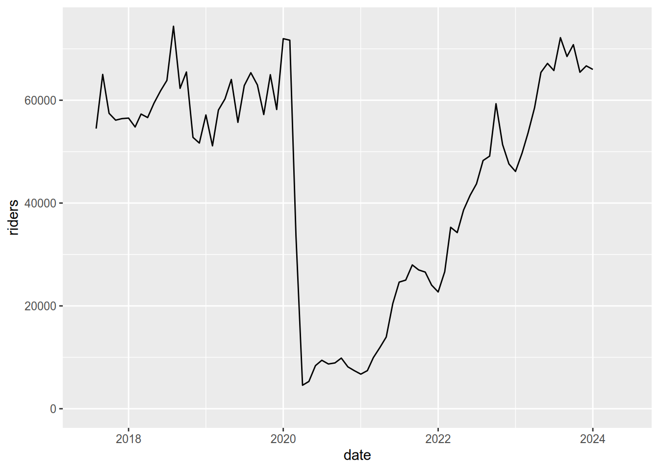

Notice the huge drop (more than 90%) in April of 2020 due to the COVID-19 pandemic!

2.1.6 Without `tidyr`

This section shows how to pivot datasets without the help of the tidyr package. In practice, we recommend that you use the package, but the examples here may make it easier to understand what’s actually happening when you pivot a dataset.

2.1.6.1 Rows into Columns

The steps for pivoting table2 wider are:

Subset rows to separate cases and population values.
Remove the type column from each.
Rename the count column to cases and population.
Merge the two subsets by matching country and year.

And the code is:

# Step 1
cases = table2[table2$type == "cases", ]
pop = table2[table2$type == "population", ]
# Step 2
cases = cases[-3]
pop = pop[-3]
# Step 3
names(cases)[3] = "cases"
names(pop)[3] = "population"
# Step 4
merge(cases, pop)

##       country year  cases population
## 1 Afghanistan 1999    745   19987071
## 2 Afghanistan 2000   2666   20595360
## 3      Brazil 1999  37737  172006362
## 4      Brazil 2000  80488  174504898
## 5       China 1999 212258 1272915272
## 6       China 2000 213766 1280428583

2.1.6.2 Columns into Rows

The steps for pivoting table4a longer are:

Subset columns to separate 1999 and 2000 into two data frames.
Add a year column to each.
Rename the 1999 and 2000 columns to cases.
Stack the two data frames with rbind.

And the code is:

# Step 1
df99 = table4a[-3]
df00 = table4a[-2]
# Step 2
df99$year = "1999"
df00$year = "2000"
# Step 3
names(df99)[2] = "cases"
names(df00)[2] = "cases"
# Step 4
rbind(df99, df00)

## # A tibble: 6 × 3
##   country      cases year 
##   <chr>        <dbl> <chr>
## 1 Afghanistan    745 1999 
## 2 Brazil       37737 1999 
## 3 China       212258 1999 
## 4 Afghanistan   2666 2000 
## 5 Brazil       80488 2000 
## 6 China       213766 2000

2.2 Relational Datasets

Many datasets contain multiple tables (or data frames) that are all closely related to each other. Sometimes, the rows in one table may be connected the rows in others through columns they have in common.

For example, our library keeps track of its books using three tables: one identifying books, one identifying borrowers, and one that records each book checkout. Each book and each borrower has a unique identification number, recorded in the book and borrower tables, respectively. These ID numbers are also recorded in the checkouts table. Using the ID numbers, you can connect rows from one table to rows in another. We call this kind of dataset a relational dataset, because there are relationships between the tables.

Storing relational datasets as several small tables rather than one large table has many benefits. Perhaps the most important is that it reduces redundancy and thereby reduces the size (in bytes) of the dataset. As a result, most databases are designed to store relational datasets.

Because the data are split across many different tables, relational datasets also pose a unique challenge: to explore, compute statistics, make visualizations, and answer questions, you’ll typically need to combine the data of interest into a single table. One way to do this is with a join, an operation that combines rows from two tables based on values of a column they have in common. There are many different types of joins, which are covered in the subsequent sections.

2.2.1 The dplyr Package

The dplyr package provides functions to join related data frames, among other things. Check out this list of all the functions provided by dplyr.

If you’ve ever used SQL, you’re probably familiar with relational datasets and recognize functions like select, left_join, and group_by. In fact, dplyr was designed to bring SQL-style data manipulation to R. As a result, many concepts of dplyr and SQL are nearly identical, and even the language overlaps a lot. I’ll point out some examples of this as we go, because I think some people might find it helpful. If you haven’t used SQL, don’t worry—all of the functions will be explained in detail.

2.2.2 Gradebook Dataset

Another example of a relational dataset that we all interact with regularly is the university gradebook. One table might store information about students and another might store their grades. The grades are linked to the student records by student ID. Looking at a student’s grades requires combining the two tables with a join.

Let’s use a made-up gradebook dataset to make the idea of joins concrete. We’ll create two tables: the first identifies students by name and ID, and the second lists their grades in a class.

# Example datasets
students = data.frame(
  student_id = c(1, 2, 3, 4),
  name = c("Angel", "Beto", "Cici", "Desmond"))

students

##   student_id    name
## 1          1   Angel
## 2          2    Beto
## 3          3    Cici
## 4          4 Desmond

grades = data.frame(
  student_id = c(2, 3, 4, 5, 6),
  grade = c(90, 85, 80, 75, 60))

grades

##   student_id grade
## 1          2    90
## 2          3    85
## 3          4    80
## 4          5    75
## 5          6    60

The rows and columns of these tables have different meanings, so we can’t stack them side-by-side or one on top of the other. The “key” piece of information for linking them is the student_id column present in both.

In relational datasets, each table usually has a primary key, a column of values that uniquely identify the rows. Key columns are important because they link rows in one table to rows in other tables.

In the gradebook dataset, student_id is the primary key for the students table. Although the values of student_id in the grades table are unique, it is not a primary key for the grades table, because a student could have grades for more than one class.

When one table’s primary key is included in another table, it’s called a foreign key. So student_id is a foreign key in the grades table.

If you’ve used SQL, you’ve probably heard the terms primary key and foreign key before. They have the same meaning in R.

In most databases, the primary key must be unique—there can be no duplicates. That said, the datasets you’ll use in R are not always coming from a database, so they may have key columns that are not unique. We’ll talk later about how to handle non-unique keys.

2.2.3 Left Joins

Suppose we want a table with each student’s name and grade. This is a combination of information from both the students table and the grades table, but how can we combine the two?

The students table contains the student names and has one row for each student. So we can use the students table as a starting point. Then we need to use each student’s ID number to look up their grade in the grades table.

When you want combine data from two tables like this, you should think of using a join. In joins terminology, the two tables are usually called the left table and right table so that it’s easy to refer to each without ambiguity.

For this particular example, we’ll use a left join. A left join keeps all of the rows in the left table and combines them with rows from the right table that match the primary key.

We want to keep every student in the students table, so we’ll use it as the left table. The grades table will be the right table. The key that links the two tables is student_id. This left join will only keep rows from the grades table that match student IDs present in the students table.

In dplyr, you can use the left_join function to carry out a left join. The first argument is the left table and the second argument is the right table. You can also set an argument for the by parameter to specify which column(s) to use as the key. Thus:

# load dplyr package
library(dplyr)

# Left join
left_join(students, grades, by = "student_id")

##   student_id    name grade
## 1          1   Angel    NA
## 2          2    Beto    90
## 3          3    Cici    85
## 4          4 Desmond    80

Note that the keys do not match up perfectly between the tables: the grades table has no rows with student_id 1 (Angel) and has rows with student_id 5 (an unknown student). Because we used a left join, the result has a missing value (NA) in the grade column for Angel and no entry for student_id 5. A left join augments the left table (students) with columns from the right table (grades). So the result of a left join will often have the same number of rows as the left table. New rows are not added for rows in the right table with non-matching key values.

There is one case where the result of a left join will have more rows than the left table: when a key value is repeated in either table. In that case, every possible match will be provided in the result. For an example, let’s add rows with repeat IDs to both the students and grades tables. Let’s also rename the student_id column of grades to be sid so we can see how to join tables where the key column names don’t match.

# Example datasets
students = data.frame(
  student_id = c(1, 2, 3, 4, 4),
  name = c("Angel", "Beto", "Cici", "Desmond", "Erik"))

grades = data.frame(
  sid = c(2, 3, 4, 5, 2),
  grade = c(90, 85, 80, 75, 60))

# Left join
left_join(students, grades, by = join_by(student_id == sid))

## Warning in left_join(students, grades, by = join_by(student_id == sid)): Detected an unexpected many-to-many relationship between `x` and `y`.
## ℹ Row 2 of `x` matches multiple rows in `y`.
## ℹ Row 3 of `y` matches multiple rows in `x`.
## ℹ If a many-to-many relationship is expected, set `relationship = "many-to-many"` to silence this warning.

##   student_id    name grade
## 1          1   Angel    NA
## 2          2    Beto    90
## 3          2    Beto    60
## 4          3    Cici    85
## 5          4 Desmond    80
## 6          4    Erik    80

Both of the tables had five rows, but the result has six rows because student_id is 4 for two rows of students and sid is 2 for two rows of grades. R warns that there is a many-to-many relationship in the join, which means that duplicate keys were matched in the left table and the right table. When there are no duplicate keys in either table, the match is one-to-one. When there are duplicates in one table only, the match is one-to-many or many-to-one. These are often desired behavior and so R just complies silently. A many-to-many match may be desired, but it is often a sign that something has gone wrong, so R emits a warning. You can get funky results when your keys are not unique!

Cats join meme

2.2.4 Other Joins

There are several other kinds of joins:

A right join is almost the same as a left join, but reverses the roles of the left and right table. All rows from the right table are augmented with columns from the left table where the key matches.
An inner join returns rows from the left and right tables only if they match (their key appears in both tables).
A full join returns all rows from the left table and from the right table, even if they do not match.

2.2.4.1 Inner Join

An inner join returns the same columns as a left join, but potentially fewer rows. The result of a inner join only includes the rows that matched according to the join specification. This will leave out some rows from the left table if they aren’t matched in the right table, which is the difference between an inner join and a left join.

# Example datasets
students = data.frame(
  student_id = c(1, 2, 3, 4, 4),
  name = c("Angel", "Beto", "Cici", "Desmond", "Erik"))

grades = data.frame(
  student_id = c(2, 3, 4, 5, 2),
  grade = c(90, 85, 80, 75, 60))

# Inner join
inner_join(students, grades, by = "student_id")

## Warning in inner_join(students, grades, by = "student_id"): Detected an unexpected many-to-many relationship between `x` and `y`.
## ℹ Row 2 of `x` matches multiple rows in `y`.
## ℹ Row 3 of `y` matches multiple rows in `x`.
## ℹ If a many-to-many relationship is expected, set `relationship = "many-to-many"` to silence this warning.

##   student_id    name grade
## 1          2    Beto    90
## 2          2    Beto    60
## 3          3    Cici    85
## 4          4 Desmond    80
## 5          4    Erik    80

Notice that the result has one row for every time the keys match, but does not include rows from either table where the keys don’t match. This is different from the left join, which retained the row for Angel from the left (students) table in the result even though it had no match in the right (grades) table.

2.2.5 Getting Clever with `join_by`

So far, we’ve focused on the join types and the tables. There’s been a third element in all of the examples that we’ve mostly ignored until now: the by argument in the joins. Specifying a single column name (like student_id) works great when the key columns have the same names in both tables. However, real examples are often more complicated. For those times, dplyr provides a function called join_by, which lets you create join specifications to solve even very complicated problems. We begin with an example where the key name in the grades table has been changed from student_id to sid.

# Example datasets
students = data.frame(
  student_id = c(1, 2, 3, 4),
  name = c("Angel", "Beto", "Cici", "Desmond"))

grades = data.frame(
  sid = c(2, 3, 4, 5),
  grade = c(90, 85, 80, 75))

# Left join
left_join(students, grades, by = join_by(student_id==sid))

##   student_id    name grade
## 1          1   Angel    NA
## 2          2    Beto    90
## 3          3    Cici    85
## 4          4 Desmond    80

Since the key column names don’t match, I have provided a join_by specification. Specifying a match via join_by is very powerful and flexible, but the main thing to recognize here is that R searches for the column name on the left of the double-equals in the left table and searches for the column name on the right of the double-equals in the right table. In this example, that means the join will try to match students$student_id to grades$sid.

2.2.5.1 Matching multiple columns

Sometimes it takes more than one key to uniquely identify a row of data. For example, suppose some of our students are retaking the class in 2023 after already taking it in 2022. Then we would need to combine the student ID with the year to uniquely identify a student’s grade. You can include multiple comparisons in a join_by specification by separating them with commas. In the following example, student ID still has different names between the tables but the year column has the same name in both tables.

In order to construct the new grades data frame, we make use of a new function from the dplyr package. The mutate function allows you to calculate columns from the existing columns of a data frame without having to write grades$ in front of each column. It is better for us here than the with function we saw earlier because we can use mutate to generate multiple columns at the same time. We also introduce rbind, which creates a new data frame by combining the rows of two (or more) data frames.

# Example datasets
students = data.frame(
  student_id = c(1, 2, 3, 4),
  name = c("Angel", "Beto", "Cici", "Desmond"))

# duplicate the students for two years
students = bind_rows(
  mutate(students, year = 2022),
  mutate(students, year = 2023)
)

# create the grades data.frame
grades = data.frame(
  sid = c(2, 3, 4, 5),
  grade = c(90, 85, 80, 75)
  )

# duplicate the grades table for two years
grades = rbind(
  mutate(grades, year = 2022, grade = grade - 50),
  mutate(grades, year = 2023)
)

# Left join
left_join(students, grades, by = join_by(student_id==sid, year))

##   student_id    name year grade
## 1          1   Angel 2022    NA
## 2          2    Beto 2022    40
## 3          3    Cici 2022    35
## 4          4 Desmond 2022    30
## 5          1   Angel 2023    NA
## 6          2    Beto 2023    90
## 7          3    Cici 2023    85
## 8          4 Desmond 2023    80

To learn clever tricks for complicated joins, see the documentation at ?join_by.

2.2.6 Examples

We’ve seen enough of the made-up grades example! Let’s look at some real data and practice our skills!

Let’s begin by looking at the data on books, borrowers, and checkouts. Download the three tables (in CSV format) via these links. Make sure you keep track of their location so tat you can import them from the location where you downloaded them.

library(readr)
borrowers = read_csv("data/library/borrowers.csv")
books = read_csv("data/library/books.csv")
checkouts = read_csv("data/library/checkouts.csv")

# show the top rows
head(books)

## # A tibble: 6 × 14
##   book_id title          author publisher creation_date       pub_date item_type
##     <dbl> <chr>          <chr>  <chr>     <dttm>              <chr>    <chr>    
## 1       1 The textual t… Boter… Brill     2016-08-03 01:02:20 1988     Book - P…
## 2       2 Intellectual … <NA>   Universi… 2016-08-03 01:02:26 ©2003.   Book - P…
## 3       3 The last redw… Leyde… Sierra C… 2016-08-03 01:02:29 [1969]   Book - P…
## 4       4 Large lakes :… <NA>   Springer… 2016-08-03 01:02:30 ©1990.   Book - P…
## 5       5 Ruling suburb… McLar… Associat… 2016-08-03 01:02:37 ©2003.   Book - P…
## 6       6 Laser diode m… Peter… Sold and… 2016-08-03 01:02:42 ©1988.   Book - P…
## # ℹ 7 more variables: location_code <chr>, material_type <chr>, barcode <dbl>,
## #   publication_place <chr>, language <chr>, descripton <chr>, loans <dbl>

head(borrowers)

## # A tibble: 6 × 3
##   borrower_id user_group        creation_date      
##         <dbl> <chr>             <dttm>             
## 1           1 Faculty and Staff 2020-04-10 00:00:00
## 2           2 Faculty and Staff 2020-05-17 00:00:00
## 3           3 Faculty and Staff 2020-05-30 00:00:00
## 4           4 Law Faculty       2020-06-05 00:00:00
## 5           5 Faculty and Staff 2020-06-19 00:00:00
## 6           6 Faculty and Staff 2020-07-08 00:00:00

head(checkouts)

## # A tibble: 6 × 5
##   book_id borrower_id barcode loan_date           due_date           
##     <dbl>       <dbl>   <dbl> <dttm>              <dttm>             
## 1    1705         129 3.12e13 2019-05-15 00:00:00 2024-06-30 00:00:00
## 2    4542         353 8.70e 6 2019-01-17 00:00:00 2022-06-30 00:00:00
## 3    2958         585 3.12e13 2022-04-06 00:00:00 2024-06-30 00:00:00
## 4     575         465 3.12e13 2020-02-16 00:00:00 2024-06-30 00:00:00
## 5    1493         425 3.12e13 2022-11-07 00:00:00 2024-06-30 00:00:00
## 6     539         522 3.12e13 2019-02-20 00:00:00 2024-06-30 00:00:00

# get the table sizes
dim(books)

## [1] 5665   14

dim(borrowers)

## [1] 722   3

dim(checkouts)

## [1] 1000    5

Suppose we want to know which books were checked out most often, or were generally checked out by the same people. The books table has a key column called book_id and the borrowers table has a primary key called borrower_id. The checkouts has two ID columns: book_id and borrower_id. These match the borrower and book IDs in the borrowers and books tables. Obviously, these aren’t unique: one person may check out multiple books, and a book can be checked out on more than one occasion.

Now we can begin to reason about how to approach the goal of identifying the books that are most often checked out. We want to augment the checkouts table with the information in the books table, matching rows where book_id matches. Every row in the checkouts table should match exactly one row in the results and every row in the results should match exactly one row in the checkouts table.

Since we want to preserve the rows of checkouts, we will do a left join, with checkouts as the left table. What to use as the right table depends on what information we want to join to the checkouts. Let’s begin by joining checkouts to books and identifying which books were checked out most often.

We are once again going to chain multiple data-processing steps together with the pipe (|>). We also introduce a few new functions from dplyr: group_by forms row groups based on the values of some column(s); summarize calculates a single-row summary that replaces all the rows in a group; n counts the rows in a group; and finally arrange puts the rows in order according to the values in some column(s).

# Top ten books with most checkouts
left_join(checkouts, books, by="book_id") |>
  group_by(book_id) |>
  summarize(title=first(title), author=first(author), n_checkouts=n()) |>
  arrange(desc(n_checkouts)) |>
  head(n=10)

## # A tibble: 10 × 4
##    book_id title                                              author n_checkouts
##      <dbl> <chr>                                              <chr>        <int>
##  1       1 "The textual tradition of Plato's Republic /"      Boter…           1
##  2      13 "Sechs italienische Sonaten : für Querflöte und B… Quant…           1
##  3      16 "Plato's moral realism : the discovery of the pre… Rist,…           1
##  4      23 "Second World War /"                               Gilbe…           1
##  5      28 "Die Fliegen der palaearktischen Region."          Lindn…           1
##  6      36 "Early English Text Society."                      <NA>             1
##  7      48 "City, chant, and the topography of early music /" <NA>             1
##  8      59 "Fiscal federalism"                                Oates…           1
##  9      67 "Armenia: cradle of civilization."                 Lang,…           1
## 10      72 "Aristotle on science, the \"Posterior analytics\… Sympo…           1

Just for fun, here is an instructive example of why relational tables are a better way to store data than putting everything into one spreadsheet. If we want to identify the authors whose books were most checked out from the UCD library, we might think to adapt our previous example to group by author rather than by book_id.

# Top ten authors with most checkouts
inner_join(checkouts, books, by="book_id") |>
  group_by(author) |>
  summarize(author=first(author), n_checkouts = n()) |>
  arrange(desc(n_checkouts)) |>
  head(n=10)

## # A tibble: 10 × 2
##    author                                  n_checkouts
##    <chr>                                         <int>
##  1 <NA>                                            224
##  2 California.                                       6
##  3 Averroës, 1126-1198.                              3
##  4 Origen.                                           3
##  5 United States Strategic Bombing Survey.           3
##  6 Agresti, Alan.                                    2
##  7 Areeda, Phillip, author.                          2
##  8 Balibar, Étienne, 1942-                           2
##  9 Burns, Catherine E.                               2
## 10 Giles, Herbert Allen, 1845-1935.                  2

The problem is that the author column is a text field for author name(s), which is not a one-to-one match to a person. There are a lot of reasons: some books have multiple authors, some authors change their names, the order of personal name and family name may be reversed, and middle initials are sometimes included, sometimes not. A table of authors would allow you to refer to authors by a unique identifier and have it always point to the same name (this is what ORCID does for scientific publishing).

2.2.6.1 Three or More Tables

A join operates on two tables, but you can combine multiple tables by doing several joins in a row. Let’s look at an example that combines checkouts, books, and borrowers in order to see how many books were checked out by students, faculty, and staff.

# list the borrowers who checked out the most books
left_join(checkouts, books, by="book_id") |>
  left_join(borrowers, by="borrower_id") |>
  group_by(borrower_id) |>
  summarize(account_type=first(user_group), n_checkouts = n()) |>
  arrange(desc(n_checkouts))

## # A tibble: 319 × 3
##    borrower_id account_type      n_checkouts
##          <dbl> <chr>                   <int>
##  1         217 Faculty and Staff          30
##  2         449 Faculty and Staff          29
##  3         524 Faculty and Staff          22
##  4         569 Faculty and Staff          21
##  5          19 Faculty and Staff          19
##  6         381 Faculty and Staff          17
##  7          20 Faculty and Staff          16
##  8         500 Faculty and Staff          15
##  9         666 Faculty and Staff          15
## 10         129 Faculty and Staff          14
## # ℹ 309 more rows

This works because the result of the first join is still a table where each row is one checkout. Keeping this as the left table, we then join the table borrowers so the result is a table where each row is one checkout, with information about both the book and the borrower. Then we can summarize the data by how many books were checked out by each type of library user.

2.2.7 Be Explicit

Do you find it odd that we have to tell R exactly what kind of data join to do by calling one of left_join, right_join, inner_join, or full_join? Why isn’t there just one function called join that assumes you’re doing a left join unless you specifically tell it otherwise like join(..., type="inner")? If you think it would be confusing for R to make assumptions about what kind of data join we want, then you’re on the right track! Watch out for these other cases where R does make strong assumptions about what the default behavior should be.

A general principle of programming is that explicit is better than implicit because writing information into your code explicitly makes it easier to understand what the code does. Here are some examples of implicit assumptions R will make unless you provide explicit instructions.

2.2.7.1 Handling Duplicate Keys

Values in the key columns may not be unique. What do you think happens when you join using keys that aren’t unique?

# Example datasets
students = data.frame(
  student_id = c(1, 2, 3, 4, 4),
  name = c("Angel", "Beto", "Cici", "Desmond", "Erik"))

grades = data.frame(student_id = c(2, 2, 3, 4, 4, 5),
                        grade = c(90, 50, 85, 80, 75, 30))

# Left join
left_join(students, grades, by = "student_id")

## Warning in left_join(students, grades, by = "student_id"): Detected an unexpected many-to-many relationship between `x` and `y`.
## ℹ Row 2 of `x` matches multiple rows in `y`.
## ℹ Row 4 of `y` matches multiple rows in `x`.
## ℹ If a many-to-many relationship is expected, set `relationship = "many-to-many"` to silence this warning.

##   student_id    name grade
## 1          1   Angel    NA
## 2          2    Beto    90
## 3          2    Beto    50
## 4          3    Cici    85
## 5          4 Desmond    80
## 6          4 Desmond    75
## 7          4    Erik    80
## 8          4    Erik    75

We get one row in the result for every possible combination of the matching keys! Sometimes that is what you want, and other times not. In this case, it might be reasonable that Beto, Desmond, and Erik have multiple grades in the book, but it is probably not reasonable that both Desmond and Erik have student ID 4 and have the same grades as each other. This is a many-to-many match, with all the risks we’ve mentioned before.

2.2.7.1.1 Specifying the Expected Relationship

You can be explicit about what kind of relationship you expect in the join by specifying the relationship parameter. Your options are one-to-one, one-to-many, or many-to-one. Any of those will stop the code with an error if the data doesn’t match the relationship you told it to expect.

If you leave the relationship parameter blank, R will allow a many-to-many join but will raise a warning. Pay attention to your warning messages! If you know in advance that you want a many-to-many join, then you can provide the argument relatonship='many-to-many', which will do the same as leaving relationship blank, except it will not raise the warning.

2.2.7.1.2 Using Only Distinct Rows

An alternative to handling duplicate keys is to subset the data to avoid duplicates in the first place. The dplyr package provides a function, distinct, which can help. When distinct finds duplicated rows, it keeps the first one.

# Example datasets
students = data.frame(
  student_id = c(1, 2, 3, 4, 4),
  name = c("Angel", "Beto", "Cici", "Desmond", "Erik"))

grades = data.frame(student_id = c(2, 2, 3, 4, 4, 5),
                        grade = c(90, 50, 85, 80, 75, 30))

# Left join
distinct_keys_result = students |> distinct(student_id, .keep_all=TRUE) |>
  left_join(grades, by = "student_id")

2.2.7.2 Ambiguous Columns

When the two tables have columns with the same names, it is ambiguous which one to use in the result. R handles that situation by keeping both but changing the names to include the table names. So the column from the left table gets a .x appended by default and the column from the right table gets a .y appended by default. Let’s see an example. Suppose that the date_created column of the borrowers table had the name date instead. Then in the joined data it would be ambiguous with the date column of the checkouts table.

# Rename the date_created column of borrowers
borrowers$date = borrowers$creation_date
checkouts$date = checkouts$loan_date

# Now create the list of checkouts
left_join(checkouts, books, by="book_id") |>
  left_join(borrowers, by="borrower_id") |>
  head(n=10)

## # A tibble: 10 × 22
##    book_id borrower_id barcode.x loan_date           due_date           
##      <dbl>       <dbl>     <dbl> <dttm>              <dttm>             
##  1    1705         129   3.12e13 2019-05-15 00:00:00 2024-06-30 00:00:00
##  2    4542         353   8.70e 6 2019-01-17 00:00:00 2022-06-30 00:00:00
##  3    2958         585   3.12e13 2022-04-06 00:00:00 2024-06-30 00:00:00
##  4     575         465   3.12e13 2020-02-16 00:00:00 2024-06-30 00:00:00
##  5    1493         425   3.12e13 2022-11-07 00:00:00 2024-06-30 00:00:00
##  6     539         522   3.12e13 2019-02-20 00:00:00 2024-06-30 00:00:00
##  7    4374         224   3.12e13 2019-05-03 00:00:00 2024-06-30 00:00:00
##  8    4234         457   3.12e13 2018-09-18 00:00:00 2024-06-30 00:00:00
##  9    3745         488   3.12e13 2021-06-08 00:00:00 2024-06-30 00:00:00
## 10    5226           4   3.11e13 2020-10-02 00:00:00 2023-06-30 00:00:00
## # ℹ 17 more variables: date.x <dttm>, title <chr>, author <chr>,
## #   publisher <chr>, creation_date.x <dttm>, pub_date <chr>, item_type <chr>,
## #   location_code <chr>, material_type <chr>, barcode.y <dbl>,
## #   publication_place <chr>, language <chr>, descripton <chr>, loans <dbl>,
## #   user_group <chr>, creation_date.y <dttm>, date.y <dttm>

If you aren’t satisfied with appending .x and .y to the ambiguous columns, then you can specify the suffix argument with a pair of strings like this:

# Now create the list of checkouts
left_join(checkouts, books, by="book_id", suffix=c("_checkout", "_book")) |>
  head(n=10)

## # A tibble: 10 × 19
##    book_id borrower_id barcode_checkout loan_date           due_date           
##      <dbl>       <dbl>            <dbl> <dttm>              <dttm>             
##  1    1705         129          3.12e13 2019-05-15 00:00:00 2024-06-30 00:00:00
##  2    4542         353          8.70e 6 2019-01-17 00:00:00 2022-06-30 00:00:00
##  3    2958         585          3.12e13 2022-04-06 00:00:00 2024-06-30 00:00:00
##  4     575         465          3.12e13 2020-02-16 00:00:00 2024-06-30 00:00:00
##  5    1493         425          3.12e13 2022-11-07 00:00:00 2024-06-30 00:00:00
##  6     539         522          3.12e13 2019-02-20 00:00:00 2024-06-30 00:00:00
##  7    4374         224          3.12e13 2019-05-03 00:00:00 2024-06-30 00:00:00
##  8    4234         457          3.12e13 2018-09-18 00:00:00 2024-06-30 00:00:00
##  9    3745         488          3.12e13 2021-06-08 00:00:00 2024-06-30 00:00:00
## 10    5226           4          3.11e13 2020-10-02 00:00:00 2023-06-30 00:00:00
## # ℹ 14 more variables: date <dttm>, title <chr>, author <chr>, publisher <chr>,
## #   creation_date <dttm>, pub_date <chr>, item_type <chr>, location_code <chr>,
## #   material_type <chr>, barcode_book <dbl>, publication_place <chr>,
## #   language <chr>, descripton <chr>, loans <dbl>

By specifying the suffix argument, we get column names in the result with more meaningful names.

2.2.7.3 Missing Values

The dplyr package has a default behavior that I think is dangerous. In the conditions of a join, NA==NA evaluates to TRUE, which is unlike the behavior anywhere else in R. This means that keys identified as NA will match other NAs in the join. This is a very strong assumption that seems to contradict the idea of a missing value since if we actually don’t know two keys, how can we say that they match? And if we know two keys have the same value then they should be labeled in the data. In my opinion, it’s a mistake to have the computer make strong assumptions by default, and especially if it does so without warning the user. Fortunately, there is a way to make the more sensible decision that NAs don’t match anything: include the argument na_matches='never' in the join.

# Example datasets
students = data.frame(
  student_id = c(1, NA, 3, 4),
  name = c("Angel", "Beto", "Cici", "Desmond"))

grades = data.frame(student_id = c(2, NA, 4, 5),
                        grade = c(90, 85, 80, 75))

# Left joins
left_join(students, grades, by = "student_id")

##   student_id    name grade
## 1          1   Angel    NA
## 2         NA    Beto    85
## 3          3    Cici    NA
## 4          4 Desmond    80

left_join(students, grades, by = "student_id", na_matches = "never")

##   student_id    name grade
## 1          1   Angel    NA
## 2         NA    Beto    NA
## 3          3    Cici    NA
## 4          4 Desmond    80

Notice that since Beto’s student ID is NA, none of the rows in the grades table can match him. As a result, his grade is left NA in the result.

2.2.8 Conclusion

You’ve now seen how to join data tables that can be linked by key columns. I encourage you to expand on the examples by posing questions and trying to write the code to answer them. Reading the documentation for join functions and join_by specifications is a great way to continue your learning journey by studying the (many!) special cases that we skipped over here.