3 Best Practices for Writing R Scripts

This chapter is all about R scripts: what they are, when to use them, and how to write them—with specific emphasis making sure your scripts are easy to read, extend, debug, and reuse. Topics covered along the way include package management, how to use iteration, how to print or log output, and how to read input from the command line or from configuration files.

Learning Objectives

After completing this session, learners should be able to:

Describe the advantages and disadvantages of using scripts
Develop modular scripts that serve as applications and libraries
Inspect and manage R’s software (package) environment
Describe and use R’s for, while, and repeat loops
Identify the most appropriate iteration strategy for a given task
Explain strategies to organize iterative code
Identify and explain the difference between R’s various printing functions
Read user input from the command line into R
Read data from configuration files into R

3.1 Introduction

An R script is a text file that contains R code. R scripts usually have the extension .R. You might already use R scripts in your workflow (for example, if you learned R from DataLab’s R Basics Workshop Series). Even if you do, this chapter covers many different practices you can adopt to use scripts more effectively. Although the chapter is focused on R, many of the practices also apply to scripting other languages.

Notebooks, which usually have the extension .Rmd, are the main alternative to scripts. Scripts and notebooks are both great ways to store code, and for most projects, DataLab staff use a mix of both. To decide which one to use, think about why you’re writing code. Compared to notebooks, the specific advantages of scripts are that they are:

Simple. Scripts are text files and usually only contain one programming language (in our case, R). Notebooks require familiarity with Markdown, and some also require special software.
Easy to reuse. In R, you can run all of the code in a script with the source function. This makes scripts a great way to create a library of reusable functions. Writing reusable scripts is also the first step towards developing packages to share with a wider audience.
Easy to run in a command-line interface. R provides a command-line program, Rscript, for running R scripts. Although you probably use a graphical interface to run code on your computer, high-performance computing environments do not always have a graphical interface, and even when they do, the default is usually a command-line interface. Running notebooks at the command-line is more difficult.

Scripts also have one big disadvantage compared to notebooks: results must be saved and viewed after the script runs, which means you have to plan ahead and write some extra code. As a result, we recommend scripts for code you plan to reuse or run at the command-line (especially if it will take a long time to run), and recommend notebooks for exploratory work. You can read more about how to decide in DataLab’s Reproducibility Principles and Practices reader.

This chapter is organized around a single case study (Section 3.2) that benefits from many of the practices we recommend. At a few points, the narrative branches off from the case study to take a closer look at a particular practice or topic in more general terms.

3.2 Case Study: U.S. Fruit Prices

The U.S. Department of Agriculture (USDA) Economic Research Service (ERS) computed national average retail prices for various fruits and vegetables in 2013, 2016, and most recently, 2020. These data provide partial insight into how much Americans must spend to eat a healthy diet with a variety of fruits and vegetables. The USDA ERS warns against using the data to compare prices across years because of differences in how products were categorized, but it can still be used to examine consumer costs in a given year.

The 2020 data are provided as per-fruit Microsoft Excel (.xlsx) files or as an all-fruits comma-separated value (CSV) file ready to use with languages such as R. Unfortunately, the 2016 and 2013 data were only distributed as per-fruit files, and the structure of these files makes extracting the data non-trivial.

The goal of this case study is to develop an R script that can read the 2016 fruit data into a single all-fruit data frame. We’ll write the script in a way that makes it easy to extend to the 2016 vegetable data or the 2013 data.

3.2.1 Setting Up the Project

There are a few things you should do every time you start working on a new project. First, create a new directory to store files related to the project. This is usually called a repository or project directory. Give the repository a descriptive name such as usda_fruit_prices.

The purpose of the repository is to keep files related to the project together, so that they’re easy to find and share. Choosing a descriptive name for the repository, and for files in general, will make it easier for others and future you to understand your work. You can read more about how to organize projects and choose names in DataLab’s Reproducibility Principles and Practices reader.

Next, create a data/ subdirectory in the repository to store data. Subdirectories are a good way to keep repositories organized, especially if you follow a naming convention. For instance, DataLab projects almost always have a data/ subdirectory to store data.

Download the zipped 2016 fruit data and save it in the data/ subdirectory. Unzip the file with a zip program or R’s own unzip function. Although the 2016 data include CSV files, these have the same structural problems as the Excel files, so we’ll focus on the Excel files.

Finally, create an R/ subdirectory in the repository to store the project’s R scripts, and make a new R script in subdirectory called extract_prices.R. You can create and open the script with RStudio or your favorite text editor.

3.2.2 Setting Up the Script

Start every script with a few comments about its purpose, usage, inputs, and outputs. These comments will serve as a blueprint for your code and as documentation. Write them before you write any code—this will help you make your ideas more concrete and keep you focused when you do start writing code.

For extract_prices.R, the goal is to extract price data from the Excel file for each fruit (or vegetable). We can extract the data to a data frame, since the data are already in a tabular format. We can have the script save the data frame as an RDS file, R’s native data format. If we want to do analysis on the data, we can use a separate script that reads the RDS file. This is a separation of concerns which ensures we can focus on the task at hand—data extraction. Summarize these ideas in comments at the beginning of extract_prices.R, by adding something like this:

# Extract a data frame of prices from USDA ERS fruit (and vegetable) price data
# Excel files. Save the data frame as an RDS file.

The key to making scripts reusable is to break computational tasks into small steps and write a short function for each step. When another script (or project) involves a similar step, you can reuse or repurpose some of the functions. This function-focused, modular development strategy also makes it easier to find and fix bugs, since you can test each function on a variety of inputs to make sure it works as intended. The strategy may also help you tackle large and complex tasks, since the component steps should be smaller and simpler, and solving one provides positive feedback. Knowing what it means for a step to be “small” takes experience, but it’s usually better to err on the side of too small rather than too large. As a rule of thumb, a function with more than one screen of code is probably trying to do too much.

Scripts you plan to run, like extract_prices.R, need some kind of starting point. Since we’re taking a function-focused approach, the starting point will be a function. There’s no standard or conventional name for a starting point function in R. Many other languages use a function called main as the starting point, so we’ll copy that convention. Add a function called main to extract_prices.R:

main = function() {
  # We'll fill this in soon!
}

Now let’s think about the steps we need to take to extract the price data. We want to extract the data from many different Excel files. If you haven’t already, open a few of the files up in a spreadsheet program to take a look at the data. The first sheet of each file contains a table with the name of the fruit and prices sorted by how the fruit was prepared. The number of rows differs between fruits, but the overall structure doesn’t seem to change, which suggests we can read and process each file in the same way. There are two things you should do when you encounter a repetitive task like this one:

Start by focusing on a single case. We’ll start by focusing exclusively on extracting the data for pears (pears 2016.xlsx).
Once you get the code working on a single case, test that the code is general enough to handle other cases, and then use iteration to run the code on all cases. You’ll learn more about iteration later in this case study and in Section 3.4.

3.2.3 Reading the Pear Data

The first step to extracting the pear data is reading the pears 2016.xlsx Excel file into R. We’ll use the read_excel function from the readxl package to read the files, since R does not provide a built-in function to read Excel files. Use the R prompt to install the package:

install.packages("readxl")

Do not add this code to the extract_prices.R script. In most cases, you should not include code to install packages in your scripts. Instead, put library calls and comments near the beginning of the script, to specify which packages are required, and leave it to the user to install them. This prevents needless, time-consuming reinstallation of packages.

We’re going to use the readxl package, so add a library call for the package near the beginning of extract_prices.R, just after the purpose comments and just before the main function:

# Extract a data frame of prices from USDA ERS fruit (and vegetable) price data
# Excel files. Save the data frame as an RDS file.

library("readxl")

# ...

We’ll add more calls to library here as we decide to use more packages. This way it’s easy for someone to see which packages are required as soon as they open the script. Putting the calls to library in alphabetical order by package name is also a good idea. You can read more about how to manage the packages a script or project requires in Section 3.3.

When developing a script, it’s often helpful to run the code, check what’s working, and make changes, repeating this process until the script is finished. Fortunately, R provides a convenient way to run an entire script: the source function. The first argument is the path to the script you want to run. In your R prompt, try sourcing extract_prices.R:

source("R/extract_prices.R")

The path is relative to R’s working directory; see this section of DataLab’s R Basics reader for details about how to change the working directory. The code above assumes the repository is the working directory. If the script was sourced correctly, R will load the readxl package and define a function main, which currently does nothing. As you add code to main and add other functions, you can source the script again to update these functions in your R session. If you’re using R Studio, you can also check the “source on save” box in the graphical user interface to make R automatically call source every time you save the script. The source function can save you time during development, but of course it’s also okay to run code by typing or pasting it into the prompt.

Take a look at the help file for the read_excel function (run ?read_excel in the R prompt). The first argument is the path to the Excel file to read. Change the code in the main function to read the pear data:

main = function() {
  read_excel("data/fruit/pears 2016.xlsx")

  # More to come...
}

Source the script and then call main in the R prompt:

main()

## New names:
## • `` -> `...2`
## • `` -> `...3`
## • `` -> `...4`
## • `` -> `...5`
## • `` -> `...6`
## • `` -> `...7`

## # A tibble: 13 × 7
##    Pears—Average retail price per pound an…¹ ...2  ...3  ...4  ...5  ...6  ...7 
##    <chr>                                     <chr> <chr> <chr> <chr> <chr> <chr>
##  1 Form                                      Aver… <NA>  Prep… Size… <NA>  Aver…
##  2 <NA>                                      <NA>  <NA>  yiel… cup … <NA>  per …
##  3 Fresh1                                    1.51… per … 0.9   0.36… poun… 0.61…
##  4 Canned                                    <NA>  <NA>  <NA>  <NA>  <NA>  <NA> 
##  5 Packed in juice2                          1.78… per … 1     0.54… poun… 0.96…
##  6 Packed in syrup or water3                 1.57… per … 0.65  0.44… poun… 1.06…
##  7 1The USDA National Nutrient Database for… <NA>  <NA>  <NA>  <NA>  <NA>  <NA> 
##  8 <NA>                                      <NA>  <NA>  <NA>  <NA>  <NA>  <NA> 
##  9 2Consumers are assumed to eat the solid … <NA>  <NA>  <NA>  <NA>  <NA>  <NA> 
## 10 <NA>                                      <NA>  <NA>  <NA>  <NA>  <NA>  <NA> 
## 11 3The syrup (or water) is discarded prior… <NA>  <NA>  <NA>  <NA>  <NA>  <NA> 
## 12 <NA>                                      <NA>  <NA>  <NA>  <NA>  <NA>  <NA> 
## 13 Source: Calculated by USDA, Economic Res… <NA>  <NA>  <NA>  <NA>  <NA>  <NA> 
## # ℹ abbreviated name:
## #   ¹`Pears—Average retail price per pound and per cup equivalent, 2016`

This returns the data in the Excel file, but there’s still a lot of cleanup to do. Since we’re eventually going to extract data about many different fruits, let’s start by getting the name of the fruit from the Excel file.

3.2.4 Getting the Fruit Name

Notice that the name of each fruit is in the top left cell (A1) of its file. The read_excel function treats the first row of cells as headers, so in the data frame, the name of the fruit is in the first column name. Create a function called get_fruit_name to get this column name:

get_fruit_name = function(sheet) {
  names(sheet)[[1]]
}

Also update the main function to save the data frame in a variable and call get_fruit_name:

main = function() {
  sheet = read_excel("data/fruit/pears 2016.xlsx")

  get_fruit_name(sheet)
  # More to come...
}

Once again, source the script and call main. The return value will be a string:

## [1] "Pears—Average retail price per pound and per cup equivalent, 2016"

This has the name of the fruit, but also some extra text. To get just the name, we need to do some string processing. We’ll use the stringr package for string processing.

Install the package and add it to the library calls at the beginning of extract_prices.R:

# Extract a data frame of prices from USDA ERS fruit (and vegetable) price data
# Excel files. Save the data frame as an RDS file.

library("readxl")
library("stringr")

# ...

We’ll use several functions from stringr, but each will be explained in context. The package provides detailed documentation as well as a cheatsheet. If you want to learn more about string processing and stringr in general, see Chapter 1 of this reader.

The name of the fruit is separated from the extra text by an em dash (the — character, which is longer than minus, the - character). We can use the str_split_fixed function to split the text into two parts at the em dash. The function’s first argument is the string to split, its second is the character on which to split (copy and paste the em dash), and its third is the number of parts. The function returns a matrix where each column corresponds to one of the split parts. In extract_prices.R, update get_fruit_name to split the text and get the first element, the fruit name:

get_fruit_name = function(sheet) {
  text = names(sheet)[[1]]
  str_split_fixed(text, "—", 2)[1, 1]
}

As usual, source the script and call main. The result is just the fruit name:

## [1] "Pears"

We’ll use the fruit name later to label the data from each file.

3.2.5 Getting the Column Names

The column names on the sheet data frame come from the first row of the file, but the actual headers of the table are in the second and third rows of the file (rows 1 and 2 of the data frame):

## # A tibble: 6 × 7
##   Pears—Average retail price per pound and…¹ ...2  ...3  ...4  ...5  ...6  ...7 
##   <chr>                                      <chr> <chr> <chr> <chr> <chr> <chr>
## 1 Form                                       Aver… <NA>  Prep… Size… <NA>  Aver…
## 2 <NA>                                       <NA>  <NA>  yiel… cup … <NA>  per …
## 3 Fresh1                                     1.51… per … 0.9   0.36… poun… 0.61…
## 4 Canned                                     <NA>  <NA>  <NA>  <NA>  <NA>  <NA> 
## 5 Packed in juice2                           1.78… per … 1     0.54… poun… 0.96…
## 6 Packed in syrup or water3                  1.57… per … 0.65  0.44… poun… 1.06…
## # ℹ abbreviated name:
## #   ¹`Pears—Average retail price per pound and per cup equivalent, 2016`

Let’s create another function, get_column_names, to convert these rows into a vector we can use as column names. Add the function to extract_prices.R, with a code to get rows 1 and 2 of the data frame:

get_column_names = function(sheet) {
  # Get rows 1 and 2, all columns.
  sheet[1:2, ]
}

As usual, update main to call the new function:

main = function() {
  sheet = read_excel("data/fruit/pears 2016.xlsx")

  fruit = get_fruit_name(sheet)
  get_column_names(sheet)
  # More to come...
}

Then source extract_prices.R and call main:

## # A tibble: 2 × 7
##   Pears—Average retail price per pound and…¹ ...2  ...3  ...4  ...5  ...6  ...7 
##   <chr>                                      <chr> <chr> <chr> <chr> <chr> <chr>
## 1 Form                                       Aver… <NA>  Prep… Size… <NA>  Aver…
## 2 <NA>                                       <NA>  <NA>  yiel… cup … <NA>  per …
## # ℹ abbreviated name:
## #   ¹`Pears—Average retail price per pound and per cup equivalent, 2016`

For each column, we need to paste the rows together. This “for each” is a hint that the task that can be solved with iteration. Before proceeding, take a moment to learn more about iteration by reading through Section 3.4. For this task, the result should be one string per column, so you can use sapply to iterate over the columns.

By setting its collapse argument, you can use R’s built-in paste function to paste together the elements of a vector together. The value of collapse is inserted between the elements. For the fruit price headers, there should be a space between the row text, so we’ll set collapse = " ". In extract_prices.R, update get_column_names, source the file, and call main:

get_column_names = function(sheet) {
  # Get rows 1 and 2, all columns.
  names = sheet[1:2, ]
  sapply(names, paste, collapse = " ")
}

## Pears—Average retail price per pound and per cup equivalent, 2016 
##                                                         "Form NA" 
##                                                              ...2 
##                                         "Average retail price NA" 
##                                                              ...3 
##                                                           "NA NA" 
##                                                              ...4 
##                                        "Preparation yield factor" 
##                                                              ...5 
##                                        "Size of a cup equivalent" 
##                                                              ...6 
##                                                           "NA NA" 
##                                                              ...7 
##                                "Average price per cup equivalent"

The result is almost right, but the paste function converts all of the missing values NA to literal text "NA". To fix this, replace all of the missing values with the empty string "" before pasting the rows together. Let’s add a call to str_trim at the end of get_column_names to trim off any excess spaces as well. Once again, update the function in extract_prices.R, source the file, and call main:

get_column_names = function(sheet) {
  # Get rows 1 and 2, all columns.
  names = sheet[1:2, ]
  # Paste together, treating NAs as empty string.
  names[is.na(names)] = ""
  names = sapply(names, paste, collapse = " ")
  # Trim off extra whitespace.
  str_trim(names)
}

## [1] "Form"                             "Average retail price"            
## [3] ""                                 "Preparation yield factor"        
## [5] "Size of a cup equivalent"         ""                                
## [7] "Average price per cup equivalent"

Notice that now two of the elements are just the empty string "". Take a look at the Excel file. Can you see why this happens? These are the two columns with units, so let’s call them units1 and units2. The numbers are to make the column names are unique. Let’s also make the other column names easier to use by converting them to lowercase with str_to_lower and replacing the spaces with underscores _ with str_replace_all. In extract_prices.R, update get_column_names, source the file, and call main:

get_column_names = function(sheet) {
  # Get rows 1 and 2, all columns.
  names = sheet[1:2, ]
  # Paste together, treating NAs as empty strings.
  names[is.na(names)] = ""
  names = sapply(names, paste, collapse = " ")
  # Trim off extra whitespace.
  names = str_trim(names)

  # Replace empty names with "unitsN"
  is_empty = names == ""
  n_empty = sum(is_empty)
  names[is_empty] = paste("units", seq_len(n_empty), sep = "")

  # Convert to lowercase and replace spaces with underscores.
  names = str_to_lower(names)
  str_replace_all(names, " +", "_")
}

## [1] "form"                             "average_retail_price"            
## [3] "units1"                           "preparation_yield_factor"        
## [5] "size_of_a_cup_equivalent"         "units2"                          
## [7] "average_price_per_cup_equivalent"

These names look good enough to use.

3.2.6 Getting the Price Data

With the fruit name and column names taken care of, now it’s time to get the actual price data. There are a few different ways to identify the rows with price data. One way is to look for entries in the second column. Let’s set up a new function, get_fruit_prices. Eventually we’ll make this function return the price data, but to get started, let’s make it return the indexes of the first and last row with entries in the second column. Add this code to extract_prices.R:

get_fruit_prices = function(sheet) {
  is_filled = !is.na(sheet[, 2])
  range(which(is_filled))
}

Then update main, source the file, and call main:

main = function() {
  sheet = read_excel("data/fruit/pears 2016.xlsx")

  fruit = get_fruit_name(sheet)
  col_names = get_column_names(sheet)

  get_fruit_prices(sheet)
}

## [1] 1 6

The first index corresponds to the header row, but we already dealt with the header in Section 3.2.5. Since the header spans two rows, we can skip it by adding 2 to the first index. The second index corresponds to the last row of prices, so it seems like this is an effective strategy for getting the price data (we can’t be completely sure until we test the strategy on other fruits).

Update get_fruit_prices and main in extract_prices.R to get the subset of rows with price data and to change the column names to the ones we computed earlier:

get_fruit_prices = function(sheet, col_names) {
  # Get all rows from first entry to last entry in column 2.
  is_filled = !is.na(sheet[, 2])
  idx = range(which(is_filled))
  prices = sheet[seq(idx[1] + 2, idx[2]), ]

  # Set column names.
  names(prices) = col_names

  prices
}


main = function() {
  sheet = read_excel("data/fruit/pears 2016.xlsx")

  fruit = get_fruit_name(sheet)
  col_names = get_column_names(sheet)

  get_fruit_prices(sheet, col_names)
}

## # A tibble: 4 × 7
##   form                      average_retail_price units1   preparation_yield_fa…¹
##   <chr>                     <chr>                <chr>    <chr>                 
## 1 Fresh1                    1.5175920102         per pou… 0.9                   
## 2 Canned                    <NA>                 <NA>     <NA>                  
## 3 Packed in juice2          1.7876110202         per pou… 1                     
## 4 Packed in syrup or water3 1.5716448654999999   per pou… 0.65                  
## # ℹ abbreviated name: ¹preparation_yield_factor
## # ℹ 3 more variables: size_of_a_cup_equivalent <chr>, units2 <chr>,
## #   average_price_per_cup_equivalent <chr>

The result looks good, but notice that the "Canned" row has a several missing values. Take a look at the original Excel file to figure out why this happens. The "Canned" row is the beginning of a subgroup of prices for canned fruit. The data frame returned by get_fruit_prices will be more convenient for analysis if we exclude the "Canned" row and instead mark the following two rows as canned. For instance, we might label their form as "Canned, packed in juice" and "Canned, packed in syrup or water".

One way to approach the subgroup labeling task is to compute the subgroup for each row, then use the split-apply pattern to process each subgroup. The "Canned" row doesn’t have an entry in the second column, so maybe we can use that to detect where each subgroup begins. You can use the is.na to find those rows, and the cumulative sum function cumsum to make the subgroup labels (since FALSE counts as 0 and TRUE counts as 1). Update get_fruit_prices in extract_prices.R to split the price data by subgroup labels, source the file, and call main:

get_fruit_prices = function(sheet, col_names) {
  # Get all rows from first entry to last entry in column 2.
  is_filled = !is.na(sheet[, 2])
  idx = range(which(is_filled))
  prices = sheet[seq(idx[1] + 2, idx[2]), ]

  # Set column names.
  names(prices) = col_names

  # Compute form subgroups.
  subgroups = cumsum(is.na(prices[, 2]))
  split(prices, subgroups)
}

## $`0`
## # A tibble: 1 × 7
##   form   average_retail_price units1    preparation_yield_factor
##   <chr>  <chr>                <chr>     <chr>                   
## 1 Fresh1 1.5175920102         per pound 0.9                     
## # ℹ 3 more variables: size_of_a_cup_equivalent <chr>, units2 <chr>,
## #   average_price_per_cup_equivalent <chr>
## 
## $`1`
## # A tibble: 3 × 7
##   form                      average_retail_price units1   preparation_yield_fa…¹
##   <chr>                     <chr>                <chr>    <chr>                 
## 1 Canned                    <NA>                 <NA>     <NA>                  
## 2 Packed in juice2          1.7876110202         per pou… 1                     
## 3 Packed in syrup or water3 1.5716448654999999   per pou… 0.65                  
## # ℹ abbreviated name: ¹preparation_yield_factor
## # ℹ 3 more variables: size_of_a_cup_equivalent <chr>, units2 <chr>,
## #   average_price_per_cup_equivalent <chr>

The result is a separate data frame for each subgroup. For each subgroup, we need to check whether the first row has an entry in the second column. If it doesn’t, then the first row is a group name (like "Canned") that should be pasted onto the other rows in the group. Add a function process_price_subgroup to extract_prices.R to do this for a single group:

process_price_subgroup = function(subgroup) {
  if (is.na(subgroup[1, 2])) {
    # First row is group name, so remove the row and paste the group name onto
    # the other rows.
    name = subgroup[[1, 1]]
    subgroup = subgroup[-1, ]
    form = str_to_lower(str_trim(subgroup$form))
    subgroup$form = paste(name, form, sep = ", ")
  }
  subgroup
}

You can use lapply to apply this function to each subgroup, and do.call with rbind to recombine the data frames. Update get_fruit_prices in extract_prices.R, source the file, and call main:

get_fruit_prices = function(sheet, col_names) {
  # Get all rows from first entry to last entry in column 2.
  is_filled = !is.na(sheet[, 2])
  idx = range(which(is_filled))
  prices = sheet[seq(idx[1] + 2, idx[2]), ]

  # Set column names.
  names(prices) = col_names

  # Compute form subgroups.
  subgroups = cumsum(is.na(prices[, 2]))
  by_subgroup = split(prices, subgroups)

  # Process each subgroup, then combine them into a single data frame.
  result = lapply(by_subgroup, process_price_subgroup)
  do.call(rbind, result)
}

## # A tibble: 3 × 7
##   form                        average_retail_price units1 preparation_yield_fa…¹
## * <chr>                       <chr>                <chr>  <chr>                 
## 1 Fresh1                      1.5175920102         per p… 0.9                   
## 2 Canned, packed in juice2    1.7876110202         per p… 1                     
## 3 Canned, packed in syrup or… 1.5716448654999999   per p… 0.65                  
## # ℹ abbreviated name: ¹preparation_yield_factor
## # ℹ 3 more variables: size_of_a_cup_equivalent <chr>, units2 <chr>,
## #   average_price_per_cup_equivalent <chr>

It seems like the script now works for single fruits!

3.2.7 Testing the Script

Let’s try a different fruit, peaches, to make sure the script is sufficiently general. In extract_prices.R, change the file loaded in main, source the script, and call main:

main = function() {
  sheet = read_excel("data/fruit/peaches 2016.xlsx")

  fruit = get_fruit_name(sheet)
  col_names = get_column_names(sheet)

  get_fruit_prices(sheet, col_names)
}

## # A tibble: 4 × 7
##   form                        average_retail_price units1 preparation_yield_fa…¹
## * <chr>                       <chr>                <chr>  <chr>                 
## 1 Fresh1                      1.6779315817         per p… 0.96                  
## 2 Canned, packed in juice2    1.8800453697999999   per p… 1                     
## 3 Canned, packed in syrup or… 1.5862877904999999   per p… 0.65                  
## 4 Canned, frozen              3.1870806846000002   per p… 1                     
## # ℹ abbreviated name: ¹preparation_yield_factor
## # ℹ 3 more variables: size_of_a_cup_equivalent <chr>, units2 <chr>,
## #   average_price_per_cup_equivalent <chr>

Uh-oh, the last row is "Canned, frozen", which doesn’t seem correct. Take a look at the Excel file for peaches to see what went wrong. The bug is that we assumed subgroups are always separated by header rows where there’s no price (like the "Canned" row). In the peaches file, the row with prices for frozen peaches is not separated this way. Looking at a few more of the files, it seems like there are only a few subgroups: Canned, Dried, Fresh, Frozen, and Juice. So let’s change the script to check specifically for these.

You can use stringr’s str_starts function to detect entries in the form column which start with one of the subgroup names. The second argument to the function is a regular expression (see Section 1.4.2), a string which describes a pattern. You can use the pipe character | in a regular expression to separate several different options. Update the code for get_fruit_prices in extract_prices.R, source the file, and call main:

get_fruit_prices = function(sheet, col_names) {
  # Get all rows from first entry to last entry in column 2.
  is_filled = !is.na(sheet[, 2])
  idx = range(which(is_filled))
  prices = sheet[seq(idx[1] + 2, idx[2]), ]

  # Set column names.
  names(prices) = col_names

  # Compute form subgroups.
  subgroup_names = "Canned|Dried|Fresh|Frozen|Juice"
  subgroups = cumsum(str_starts(prices$form, subgroup_names))
  by_subgroup = split(prices, subgroups)

  # Process each subgroup, then combine them into a single data frame.
  result = lapply(by_subgroup, process_price_subgroup)
  do.call(rbind, result)
}

## # A tibble: 4 × 7
##   form                        average_retail_price units1 preparation_yield_fa…¹
## * <chr>                       <chr>                <chr>  <chr>                 
## 1 Fresh1                      1.6779315817         per p… 0.96                  
## 2 Canned, packed in juice2    1.8800453697999999   per p… 1                     
## 3 Canned, packed in syrup or… 1.5862877904999999   per p… 0.65                  
## 4 Frozen                      3.1870806846000002   per p… 1                     
## # ℹ abbreviated name: ¹preparation_yield_factor
## # ℹ 3 more variables: size_of_a_cup_equivalent <chr>, units2 <chr>,
## #   average_price_per_cup_equivalent <chr>

This appears to be correct. Test the script on the pears data again as well, to make sure the changes didn’t introduce other bugs:

## # A tibble: 3 × 7
##   form                        average_retail_price units1 preparation_yield_fa…¹
## * <chr>                       <chr>                <chr>  <chr>                 
## 1 Fresh1                      1.5175920102         per p… 0.9                   
## 2 Canned, packed in juice2    1.7876110202         per p… 1                     
## 3 Canned, packed in syrup or… 1.5716448654999999   per p… 0.65                  
## # ℹ abbreviated name: ¹preparation_yield_factor
## # ℹ 3 more variables: size_of_a_cup_equivalent <chr>, units2 <chr>,
## #   average_price_per_cup_equivalent <chr>

Some of the columns in the data frame have inappropriate data types. This can be fixed with just a few lines of code, but since it doesn’t provide any additional insight into how to write scripts, we won’t do so here. If you want to know more about how to fix “messy data” problems, read Chapter 1.

3.2.8 Iterating Over All Fruit

The final step in extracting the fruit price data is to modify extract_prices.R to extract the prices of all fruits. This is also a good time to make several small changes to the script that will make it more convenient to use.

First, change the name of main to read_price_file, make the path to the Excel file a parameter called path, and limit the Excel sheet to seven columns:

read_price_file = function(path) {
  sheet = read_excel(path)
  sheet = sheet[, 1:7]

  fruit = get_fruit_name(sheet)
  col_names = get_column_names(sheet)

  prices = get_fruit_prices(sheet, col_names)
  prices$fruit = fruit
  prices
}

This change makes it possible to reuse the function for many different fruit (and vegetable) Excel files.

Next, let’s create a new main function, which will call read_price_file on all of the Excel files in a user-specified directory. The function should have two parameters: input_dir, for the path to the directory that contains the Excel files, and output_path, for a path to an RDS file where the resulting data frame should be saved. You can use list.files to get a vector of paths to all files in the input directory, lapply to iterate over the files, and saveRDS to save the result. Here’s the code to add to extract_prices.R:

main = function(
  input_dir = "data/fruit/",
  output_path = "prices.rds"
) {
  # Get vector of all files in directory.
  message("Input directory: ", input_dir)
  paths = list.files(input_dir, pattern = "*.xlsx", full.names = TRUE)

  # Read each file and combine the resulting data frames.
  result = lapply(paths, function(path) {
    message("Reading: ", path)
    read_price_file(path)
  })
  result = do.call(rbind, result)

  # Save the result to an RDS file.
  saveRDS(result, output_path)
  message("Wrote:", output_path)

  result
}

The code for the function includes several calls to message to print informational messages. It’s a good idea to include these so that you (or other users) can verify that the paths to files are correct and can quickly diagnose any bugs you encounter. You can read more about various ways to print output in R in Section 3.5.

Once again, test that the code works by sourcing the script and calling main:

## # A tibble: 62 × 8
##    form                       average_retail_price units1 preparation_yield_fa…¹
##    <chr>                      <chr>                <chr>  <chr>                 
##  1 Fresh1                     1.6155336441000001   per p… 0.9                   
##  2 Applesauce2                1.0491006433000001   per p… 1                     
##  3 Juice, ready to drink3     0.63113252779999995  per p… 1                     
##  4 Frozen4                    0.51046574550000001  per p… 1                     
##  5 Fresh1                     3.0871378169999999   per p… 0.93                  
##  6 Canned, packed in juice2   1.4742760156000001   per p… 1                     
##  7 Canned, packed in syrup, … 1.8552908088         per p… 0.65                  
##  8 Dried4                     7.3309645323000003   per p… 1                     
##  9 Fresh1                     0.54941729279999996  per p… 0.64                  
## 10 Frozen1                    3.63694066           per p… 1                     
## # ℹ 52 more rows
## # ℹ abbreviated name: ¹preparation_yield_factor
## # ℹ 4 more variables: size_of_a_cup_equivalent <chr>, units2 <chr>,
## #   average_price_per_cup_equivalent <chr>, fruit <chr>

This looks almost perfect. There are still a few minor issues with data types, and also a small bug (related to frozen juice), but all of these can be fixed with small changes to the script.

3.3 Managing Environments

Your computing environment is the collection of hardware and software you use to run code. Code developed for one computing environment will not necessarily run correctly in another. Scripting languages like R and Python are designed to work with a wide variety of hardware, so in the context of these languages, software, especially package versions, are the primary cause of incompatibility.

Documenting the computing environment your code was designed for is an important part of making your research (or other work) reproducible. One way to do this is to maintain documentation that lists the specific packages your code depends on, with complete version information.

You can get version information about your R environment with the sessionInfo function:

sessionInfo()

## R version 4.3.2 (2023-10-31)
## Platform: x86_64-pc-linux-gnu (64-bit)
## Running under: Arch Linux
## 
## Matrix products: default
## BLAS:   /usr/lib/libblas.so.3.12.0 
## LAPACK: /usr/lib/liblapack.so.3.12.0
## 
## locale:
##  [1] LC_CTYPE=en_US.UTF-8       LC_NUMERIC=C              
##  [3] LC_TIME=en_US.UTF-8        LC_COLLATE=en_US.UTF-8    
##  [5] LC_MONETARY=en_US.UTF-8    LC_MESSAGES=en_US.UTF-8   
##  [7] LC_PAPER=en_US.UTF-8       LC_NAME=C                 
##  [9] LC_ADDRESS=C               LC_TELEPHONE=C            
## [11] LC_MEASUREMENT=en_US.UTF-8 LC_IDENTIFICATION=C       
## 
## time zone: US/Pacific
## tzcode source: system (glibc)
## 
## attached base packages:
## [1] stats     graphics  grDevices utils     datasets  methods   base     
## 
## other attached packages:
## [1] stringr_1.5.1 readxl_1.4.3 
## 
## loaded via a namespace (and not attached):
##  [1] vctrs_0.6.5      cli_3.6.2        knitr_1.45       rlang_1.1.2     
##  [5] xfun_0.41        stringi_1.8.3    jsonlite_1.8.8   glue_1.6.2      
##  [9] htmltools_0.5.7  sass_0.4.8       fansi_1.0.6      rmarkdown_2.25  
## [13] cellranger_1.1.0 evaluate_0.23    jquerylib_0.1.4  tibble_3.2.1    
## [17] fastmap_1.1.1    yaml_2.3.8       lifecycle_1.0.4  bookdown_0.37   
## [21] compiler_4.3.2   pkgconfig_2.0.3  digest_0.6.34    R6_2.5.1        
## [25] utf8_1.2.4       pillar_1.9.0     magrittr_2.0.3   bslib_0.6.1     
## [29] tools_4.3.2      cachem_1.0.8

Documentation is often neglected, and it’s easy to forget that you updated a package, so you might prefer a more automated approach to recording your R environment. The renv package provides functions to record and recreate environments. See the package documentation for details about how to use the package.

3.4 Iteration Strategies

R is powerful tool for automating tasks that have repetitive steps. For example, you can:

Apply a transformation to an entire column of data.
Compute distances between all pairs from a set of points.
Read a large collection of files from disk in order to combine and analyze the data they contain.
Simulate how a system evolves over time from a specific set of starting parameters.
Scrape data from many pages of a website.

You can implement concise, efficient solutions for these kinds of tasks in R by using iteration, which means repeating a computation many times. R provides four different strategies for writing iterative code:

Vectorization, where a function is implicitly called on each element of a vector. See this section of DataLab’s R Basics reader for more details.
Apply functions, where a function is explicitly called on each element of a vector or array. See this section of DataLab’s R Basics reader for more details.
Loops, where an expression is evaluated repeatedly until some condition is met.
Recursion, where a function calls itself.

Vectorization is the most efficient and most concise iteration strategy, but also the least flexible, because it only works with vectorized functions and vectors. Apply functions are more flexible—they work with any function and any data structure with elements—but less efficient and less concise. Loops and recursion provide the most flexibility but are the least concise. In recent versions of R, apply functions and loops are similar in terms of efficiency. Recursion tends to be the least efficient iteration strategy in R.

The rest of this section explains how to write loops and how to choose which iteration strategy to use. We assume you’re already comfortable with vectorization and have at least some familiarity with apply functions.

3.4.1 For-loops

A for-loop evaluates an expression once for each element of a vector or list. The for keyword creates a for-loop. The syntax is:

for (I in DATA) {
  # Your code goes here
}

The variable I is called an induction variable. At the beginning of each iteration, I is assigned the next element of DATA. The loop iterates once for each element, unless a keyword instructs R to exit the loop early (more about this in Section 3.4.4). As with if-statements and functions, the curly braces { } are only required if the body contains multiple lines of code. Here’s a simple for-loop:

for (i in 1:10)
  message("Hi from iteration  ", i)

## Hi from iteration  1

## Hi from iteration  2

## Hi from iteration  3

## Hi from iteration  4

## Hi from iteration  5

## Hi from iteration  6

## Hi from iteration  7

## Hi from iteration  8

## Hi from iteration  9

## Hi from iteration  10

When some or all of the iterations in a task depend on results from prior iterations, loops tend to be the most appropriate iteration strategy. For instance, loops are a good way to implement time-based simulations or compute values in recursively defined sequences.

As a concrete example, suppose you want to compute the result of starting from the value 1 and composing the sine function 100 times:

result = 1
for (i in 1:100) {
  result = sin(result)
}

result

## [1] 0.1688525

Unlike other iteration strategies, loops don’t return a result automatically. It’s up to you to use variables to store any results you want to use later. If you want to save a result from every iteration, you can use a vector or a list indexed on the iteration number:

n = 1 + 100
result = numeric(n)
result[1] = 1
for (i in 2:n) {
  result[i] = sin(result[i - 1])
}

plot(result)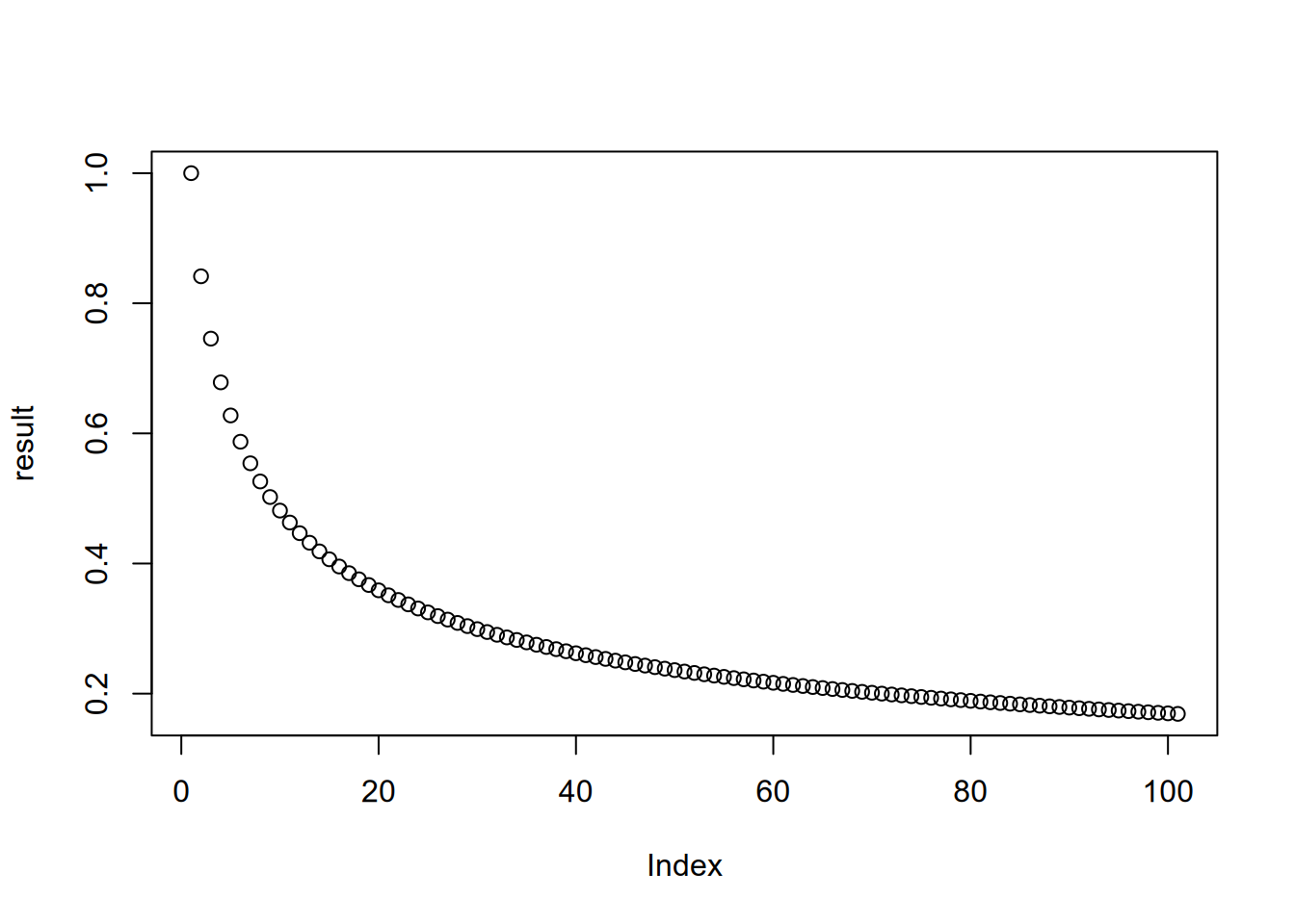

Section 3.4.3 explains this in more detail.

If the iterations in a task are not dependent, it’s preferable to use vectorization or apply functions instead of a loop. Vectorization is more efficient, and apply functions are usually more concise.

In some cases, you can use vectorization to handle a task even if the iterations are dependent. For example, you can use vectorized exponentiation and the sum function to compute the sum of the cubes of many numbers:

numbers = c(10, 3, 100, -5, 2, 10)
sum(numbers^3)

## [1] 1001910

3.4.2 While-loops

A while-loop runs a block of code repeatedly as long as some condition is TRUE. The while keyword creates a while-loop. The syntax is:

while (CONDITION) {
  # Your code goes here
}

The CONDITION should be a scalar logical value or an expression that returns one. At the beginning of each iteration, R checks the CONDITION and exits the loop if it’s FALSE. As always, the curly braces { } are only required if the body contains multiple lines of code. Here’s a simple while-loop:

i = 0
while (i < 10) {
  i = i + 1
  message("Hello from iteration ", i)
}

## Hello from iteration 1

## Hello from iteration 2

## Hello from iteration 3

## Hello from iteration 4

## Hello from iteration 5

## Hello from iteration 6

## Hello from iteration 7

## Hello from iteration 8

## Hello from iteration 9

## Hello from iteration 10

Notice that this example does the same thing as the simple for-loop in Section 3.4.1, but requires 5 lines of code instead of 2. While-loops are a generalization of for-loops, and only do the bare minimum necessary to iterate. They tend to be most useful when you don’t know how many iterations will be necessary to complete a task.

As an example, suppose you want to add up the integers in order until the total is greater than 50:

total = 0
i = 1
while (total < 50) {
  total = total + i
  message("i is ", i, " total is ", total)
  i = i + 1
}

## i is 1 total is 1

## i is 2 total is 3

## i is 3 total is 6

## i is 4 total is 10

## i is 5 total is 15

## i is 6 total is 21

## i is 7 total is 28

## i is 8 total is 36

## i is 9 total is 45

## i is 10 total is 55

total

## [1] 55

## [1] 11

3.4.3 Saving Multiple Results

Loops often produce a different result for each iteration. If you want to save more than one result, there are a few things you must do.

First, set up an index vector. The index vector should usually correspond to the positions of the elements in the data you want to process. The seq_along function returns an index vector when passed a vector or list. For instance:

numbers = c(-1, 21, 3, -8, 5)
index = seq_along(numbers)

The loop will iterate over the index rather than the input, so the induction variable will track the current iteration number. On the first iteration, the induction variable will be 1, on the second it will be 2, and so on. Then you can use the induction variable and indexing to get the input for each iteration.

Second, set up an empty output vector or list. This should usually also correspond to the input, or one element longer (the extra element comes from the initial value). R has several functions for creating vectors:

logical, integer, numeric, complex, and character create an empty vector with a specific type and length
vector creates an empty vector with a specific type and length
rep creates a vector by repeating elements of some other vector

Empty vectors are filled with FALSE, 0, or "", depending on the type of the vector. Here are some examples:

logical(3)

## [1] FALSE FALSE FALSE

numeric(4)

## [1] 0 0 0 0

rep(c(1, 2), 2)

## [1] 1 2 1 2

Let’s create an empty numeric vector congruent to the numbers vector:

n = length(numbers)
result = numeric(n)

As with the input, you can use the induction variable and indexing to set the output for each iteration.

Creating a vector or list in advance to store something, as we’ve just done, is called preallocation. Preallocation is extremely important for efficiency in loops. Avoid the temptation to use c or append to build up the output bit by bit in each iteration.

Finally, write the loop, making sure to get the input and set the output. As an example, this loop adds each element of numbers to a running total and squares the new running total:

for (i in index) {
  prev = if (i > 1) result[i - 1] else 0
  result[i] = (numbers[i] + prev)^2
}
result

## [1] 1.000000e+00 4.840000e+02 2.371690e+05 5.624534e+10 3.163538e+21

3.4.4 Break & Next

The break keyword causes a loop to immediately exit. It only makes sense to use break inside of an if-statement.

For example, suppose you want to print each string in a vector, but stop at the first missing value. You can do this with a for-loop and the break keyword:

my_messages = c("Hi", "Hello", NA, "Goodbye")

for (msg in my_messages) {
  if (is.na(msg))
    break

  message(msg)
}

## Hi

## Hello

The next keyword causes a loop to immediately go to the next iteration. As with break, it only makes sense to use next inside of an if-statement.

Let’s modify the previous example so that missing values are skipped, but don’t cause printing to stop. Here’s the code:

for (msg in my_messages) {
  if (is.na(msg))
    next

  message(msg)
}

## Hi

## Hello

## Goodbye

These keywords work with both for-loops and while-loops.

3.4.5 Planning for Iteration

At first it may seem difficult to decide if and what kind of iteration to use. Start by thinking about whether you need to do something over and over. If you don’t, then you probably don’t need to use iteration. If you do, then try iteration strategies in this order:

Vectorization
Apply functions
- Try an apply function if iterations are independent.
Loops
- Try a for-loop if some iterations depend on others.
- Try a while-loop if the number of iterations is unknown.
Recursion (which isn’t covered here)
- Convenient for naturally recursive tasks (like Fibonacci), but often there are faster solutions.

Start by writing the code for just one iteration. Make sure that code works; it’s easy to test code for one iteration.

When you have one iteration working, then try using the code with an iteration strategy (you will have to make some small changes). If it doesn’t work, try to figure out which iteration is causing the problem. One way to do this is to use message to print out information. Then try to write the code for the broken iteration, get that iteration working, and repeat this whole process.

3.4.6 Case Study: The Collatz Conjecture

The Collatz Conjecture is a conjecture in math that was introduced in 1937 by Lothar Collatz and remains unproven today, despite being relatively easy to explain. Here’s a statement of the conjecture:

Start from any positive integer. If the integer is even, divide by 2. If the integer is odd, multiply by 3 and add 1.

If the result is not 1, repeat using the result as the new starting value.

The result will always reach 1 eventually, regardless of the starting value.

The sequences of numbers this process generates are called Collatz sequences. For instance, the Collatz sequence starting from 2 is 2, 1. The Collatz sequence starting from 12 is 12, 6, 3, 10, 5, 16, 8, 4, 2, 1.

You can use iteration to compute the Collatz sequence for a given starting value. Since each number in the sequence depends on the previous one, and since the length of the sequence varies, a while-loop is the most appropriate iteration strategy:

n = 5
i = 0
while (n != 1) {
  i = i + 1
  if (n %% 2 == 0) {
    n = n / 2
  } else {
    n = 3 * n + 1
  }
  message(n, " ", appendLF = FALSE)
}

## 16 8 4 2 1

As of 2020, scientists have used computers to check the Collatz sequences for every number up to approximately \(2^{64}\). For more details about the Collatz Conjecture, check out this video.

For another example, see Liza Wood’s Real-world Function Writing Mini-reader.

3.5 Printing Output

This section introduces several different functions for printing output and making that output easier to read.

3.5.1 The `print` Function

The print function prints a string representation of an object to the console. The string representation is usually formatted in a way that exposes details important to programmers rather than users.

For example, when printing a vector, the function prints the position of the first element on each line in square brackets [ ]:

print(1:100)

##   [1]   1   2   3   4   5   6   7   8   9  10  11  12  13  14  15  16  17  18
##  [19]  19  20  21  22  23  24  25  26  27  28  29  30  31  32  33  34  35  36
##  [37]  37  38  39  40  41  42  43  44  45  46  47  48  49  50  51  52  53  54
##  [55]  55  56  57  58  59  60  61  62  63  64  65  66  67  68  69  70  71  72
##  [73]  73  74  75  76  77  78  79  80  81  82  83  84  85  86  87  88  89  90
##  [91]  91  92  93  94  95  96  97  98  99 100

The print function also prints quotes around strings:

print("Hi")

## [1] "Hi"

These features make the print function ideal for printing information when you’re trying to understand some code or diagnose a bug. On the other hand, these features also make print a bad choice for printing output or status messages for users (including you).

R calls the print function automatically anytime a result is returned at the prompt. Thus it’s not necessary to call print to print something when you’re working directly in the console—only from within loops, functions, scripts, and other code that runs non-interactively.

The print function is an S3 generic (see Section 6.4), so you if you create an S3 class, you can define a custom print method for it. For S4 objects, R uses the S4 generic show instead of print.

3.5.2 The `message` Function

To print output for users, the message function is the one you should use. The main reason for this is that the message function is part of R’s conditions system for reporting status information as code runs. This makes it easier for other code to detect, record, respond to, or suppress the output (see Section 4.2 to learn more about R’s conditions system).

The message function prints its argument(s) and a newline to the console:

message("Hello world!")

## Hello world!

If an argument isn’t a string, the function automatically and silently attempts to coerce it to one:

message(4)

## 4

Some types of objects can’t be coerced to a string:

message(sqrt)

## Error in FUN(X[[i]], ...): cannot coerce type 'builtin' to vector of type 'character'

For objects with multiple elements, the function pastes together the string representations of the elements with no separators in between:

x = c(1, 2, 3)
message(x)

## 123

Similarly, if you pass the message function multiple arguments, it pastes them together with no separators:

name = "R"
message("Hi, my name is ", name, " and x is ", x)

## Hi, my name is R and x is 123

This is a convenient way to print names or descriptions alongside values from your code without having to call a formatting function like paste.

You can make the message function print something without adding a newline at the end by setting the argument appendLF = FALSE. The difference can be easy to miss unless you make several calls to message, so the say_hello function in this example calls message twice:

say_hello = function(appendLF) {
  message("Hello", appendLF = appendLF)
  message(" world!")
}

say_hello(appendLF = TRUE)

## Hello

##  world!

say_hello(appendLF = FALSE)

## Hello world!

Note that RStudio always adds a newline in front of the prompt, so making an isolated call to message with appendLF = FALSE appears to produce the same output as with appendLF = TRUE. This is an example of a situation where RStudio leads you astray: in an ordinary R console, the two are clearly different.

3.5.3 The `cat` Function

The cat function, whose name stands for “concatenate and print,” is a low-level way to print output to the console or a file. The message function prints output by calling cat, but cat is not part of R’s conditions system.

The cat function prints its argument(s) to the console. It does not add a newline at the end:

cat("Hello")

## Hello

As with message, RStudio hides the fact that there’s no newline if you make an isolated call to cat.

The cat function coerces its arguments to strings and concatenates them. By default, a space is inserted between arguments and their elements:

cat(4)

## 4

cat(x)

## 1 2 3

cat("Hello", "Nick")

## Hello Nick

You can set the sep parameter to control the separator cat inserts:

cat("Hello", "world", x, sep = "|")

## Hello|world|1|2|3

If you want to write output to a file rather than to the console, you can call cat with the file parameter set. However, it’s preferable to use functions tailored to writing specific kinds of data, such as writeLines (for text) or write.table (for tabular data), since they provide additional options to control the output.

Many scripts and packages still use cat to print output, but the message function provides more flexibility and control to people running the code. Thus it’s generally preferable to use message in new code. Nevertheless, there are a few specific cases where cat is useful—for example, if you want to pipe data to a UNIX shell command. See ?cat for details.

3.5.4 Formatting Output

R provides a variety of ways to format data before you print it. Taking the time to format output carefully makes it easier to read and understand, as well as making your scripts seem more professional.

3.5.4.1 Escape Sequences

One way to format strings is by adding (or removing) escape sequences. An escape sequence is a sequence of characters that represents some other character, usually one that’s invisible (such as whitespace) or doesn’t appear on a standard keyboard.

In R, escape sequences always begin with a backslash. For example, \n is a newline. The message and cat functions automatically convert escape sequences to the characters they represent:

x = "Hello\nworld!"
message(x)

## Hello
## world!

The print function doesn’t convert escape sequences:

print(x)

## [1] "Hello\nworld!"

Some escape sequences trigger special behavior in the console. For example, ending a line with a carriage return \r makes the console print the next line over the line. Try running this code in a console (it’s not possible to see the result in a static book):

# Run this in an R console.
for (i in 1:10) {
  message(i, "\r", appendLF = FALSE)
  # Wait 0.5 seconds.
  Sys.sleep(0.5)
}

You can find a complete list of escape sequences in ?Quotes.

3.5.4.2 Formatting Functions

You can use the sprintf function to apply specific formatting to values and substitute them into strings. The function uses a mini-language to describe the formatting and substitutions. The sprintf function (or something like it) is available in many programming languages, so being familiar with it will serve you well on your programming journey.

The key idea is that substitutions are marked by a percent sign % and a character. The character indicates the kind of data to be substituted: s for strings, i for integers, f for floating point numbers, and so on.

The first argument to sprintf must be a string, and subsequent arguments are values to substitute into the string (from left to right). For example:

sprintf("My age is %i, and my name is %s", 32, "Nick")

## [1] "My age is 32, and my name is Nick"

You can use the mini-language to do things like specify how many digits to print after a decimal point. Format settings for a substituted value go between the percent sign % and the character. For instance, here’s how to print pi with 2 digits after the decimal:

sprintf("%.2f", pi)

## [1] "3.14"

You can learn more by reading ?sprintf.

Much simpler are the paste and paste0 functions, which coerce their arguments to strings and concatenate (or “paste together”) them. The paste function inserts a space between each argument, while the paste0 function doesn’t:

paste("Hello", "world")

## [1] "Hello world"

paste0("Hello",  "world")

## [1] "Helloworld"

You can control the character inserted between arguments with the sep parameter.

By setting an argument for the collapse parameter, you can also use the paste and paste0 functions to concatenate the elements of a vector. The argument to collapse is inserted between the elements. For example, suppose you want to paste together elements of a vector inserting a comma and space , in between:

paste(1:3, collapse = ", ")

## [1] "1, 2, 3"

Members of the R community have developed many packages to make formatting strings easier:

cli – helper functions for developing command-line interfaces, including functions to add color, progress bars, and more.
glue – alternatives to sprintf for string iterpolation.
stringr – a collection of general-purpose string manipulation functions.

3.5.5 Logging Output

Logging means saving the output from some code to a file as the code runs. The file where the output is saved is called a log file or log, but this name isn’t indicative of a specific format (unlike, say, a “CSV file”).

It’s a good idea to set up some kind of logging for any code that takes more than a few minutes to run, because then if something goes wrong you can inspect the log to diagnose the problem. Think of any output that’s not logged as ephemeral: it could disappear if someone reboots the computer, or there’s a power outage, or some other, unforeseen event.

R’s built-in tools for logging are rudimentary, but members of the community have developed a variety of packages for logging. Here are a few that are still actively maintained as of January 2023:

logger – a relatively new package that aims to improve aspects of other logging packages that R users find confusing.
futile.logger – a popular, mature logging package based on Apache’s Log4j utility and on R idioms.
logging – a mature logging package based on Python’s logging module.
loggit – integrates with R’s conditions system and writes logs in JavaScript Object Notation (JSON) format so they are easy to inspect programmatically.
log4r – another package based on Log4j with an object-oriented programming approach.

3.6 Reading Input

This section explains how to make R read inputs from the command line, configuration files, and interactive prompts. These kinds of inputs are often important for scripts, because they allow for flexibility in initial parameters and how run-time events are handled.

3.6.1 Command Line Arguments

When you run an R script from the command line, you can optionally pass additional arguments to the script by putting them after command. Command line arguments are a convenient and relatively safe way to set parameters in scripts. This is in contrast to editing scripts directly, which may be difficult (if the code is complex or disorganized) and may introduce bugs. That said, for scripts with lots of parameters, we recommend reading the parameters from a configuration file (see Section 3.6.2) instead or in addition to command line arguments.

You can capture command line arguments with R’s built-in the commandArgs function or with functions from a variety of packages. By default, the commandArgs function returns the entire command used to run R, including the Rscript command and the name of the script. You can get just the arguments after the name of the script by setting trailingOnly = TRUE. The function assumes arguments are space-separated and returns a character vector with one element for each argument. As an example, set up a script called hello_name.R:

main = function(
  args = commandArgs(trailingOnly = TRUE)
) {
  if (length(args) < 1)
    message("Usage: Rscript hello_name.R NAME")

  message("Hello, ", args[[1]], "!")
}

main()

Try running the script from the command line with this command:

Rscript hello_name.R Susan

## Hello, Susan!

Several packages on CRAN provide functions for more complex processing of command line arguments. As of 2024, many of these packages appear to be unmaintained or have undesirable dependencies (for example, the argparse package depends on Python). One of the more promising packages is optparse.

3.6.2 Configuration Files

When a script has lots of parameters, reading them from a separate configuration file is often a good idea. Configuration files are beneficial because they provide a record of parameter settings that can be saved separately from the code (with command line arguments, it’s easy to forget which settings you used in earlier runs).

There are many different formats available for configuration files. Two that are especially popular are:

Yet Another Markup Language (YAML) – YAML is a plain text format designed to be easy for people to read. It’s widely used in the R community. For instance, R Markdown notebooks typically include a YAML header for settings. The yaml package provides functions to read and write YAML files.
Tom’s Obvious Markup Language (TOML) – TOML is also a plain text format designed to be easy for people to read. Compared to YAML, TOML’s main advantage is that its syntax is simpler and thus easier to learn. TOML is widely used in other programming communities (especially Python and Rust), but is not yet widely used in the R community. The RcppTOML package provides functions to read TOML files.

3.6.3 Prompts

Sometimes it’s useful to prompt the user for input while code is running. For instance, a script that produces output can prompt the user about what to do if the output would overwrite an existing file. You can also use prompts to develop interactive programs, which may be more accessible to users unfamiliar with programming and command line interfaces.

One way to prompt the user for input is with R’s built-in readline function. The function prompts the user for input and returns whatever they enter as a string. Try out the readline function in an R prompt:

readline()

A more sophisticated way to prompt the user for input is with R’s built-in scan function. The scan function attempts to read a specific type of data, which you can customize. By default, the function prompts the user for numbers and returns when they enter a blank line. The result is a vector with one element for each number they entered. Try out the scan function in an R prompt:

result = scan()

You can set the what parameter in scan to specify the type of data to read. For instance, if you want to read strings (into a character vector), set what = character():

scan(what = character())

The scan function has many other parameters, which you can use to control things like how many values the user can enter and which values should be interpreted as the missing value NA.