12. Classification and Feature Engineering#
This chapter demonstrates how to apply what we’ve learned so far about document annotation to build a text classifier. Our emphasis will be on engineering features for a model. While, in NLP, token counts are often sufficient for various tasks, there are other features we can use to represent information about our texts; document annotation gives us a way to create them.
We’ll work with a small corpus to test out some of these features. Admittedly, the documents therein are a bit of a weird mix: our corpus is comprised of ~50 Sherlock Holmes short stories (courtesy of the McGill txtLAB), 100 movie summaries from the CMU Movie Summary Corpus, and 100 PLOS ONE biomedical abstracts. Why such a disparate corpus? Well, our focus here is on how different approaches to feature engineering might help you partition texts in your own corpora, so our intent is less about showing you a completely real word situation and more about outlining a few options you might pursue when using NLP methods in your research.
Learning objectives
By the end of this chapter, you will be able to:
Build a naive Bayes text classification model
Recognize whether a model might be overfitted
Identify possible feature sets to engineer for text data
Engineer those features using
spaCy’s document annotation modelValidate your engineered features
12.1. Preliminaries#
These are the libraries you will need for this chapter.
from pathlib import Path
import json
from collections import Counter
import spacy
from spacy.tokens import Doc
import numpy as np
import pandas as pd
from sklearn.model_selection import train_test_split
from sklearn.metrics import classification_report
from sklearn.naive_bayes import GaussianNB, MultinomialNB
from sklearn.preprocessing import MinMaxScaler
import matplotlib.pyplot as plt
import seaborn as sns
We’ll also set up an input directory and our model.
indir = Path("data/section_two/s2")
nlp = spacy.load('en_core_web_md')
And we’ll load a document manifest.
manifest = pd.read_csv(indir.joinpath("manifest.csv"), index_col = 0)
manifest.info()
<class 'pandas.core.frame.DataFrame'>
Index: 256 entries, 0 to 255
Data columns (total 3 columns):
 #   Column     Non-Null Count  Dtype
---  ------     --------------  -----
 0   file_name  256 non-null    object
 1   label      256 non-null    object
 2   label_int  256 non-null    int64
dtypes: int64(1), object(2)
memory usage: 8.0+ KB
Finally, we’ll load our corpus. Our corpus documents have already been
annotated with the model above and saved as JSON files. A corpus of this size
makes this a reasonable storage solution, though spaCy recommends looking to
Dask or Spark for bigger datasets. The code below shows you
how to load our documents. Note that you need to have the model vocabulary
to do this.
def load_doc(path):
    """Load a json file as a spaCy doc."""
    with path.open('r') as fin:
        feats = json.load(fin)
        doc = Doc(nlp.vocab).from_json(feats)

        return doc

docs = []
for fname in manifest['file_name']:
    doc = load_doc(indir.joinpath(f"input/{fname}"))
    docs.append(doc)
12.2. Modeling I#
12.2.1. Tf-idf vectors#
Before we begin feature engineering, we’ll build a baseline model against which
to compare those features. Our comparison model will be one built with tf-idf
vectors. These vectors are the product of fitting a scikit-learn
TfidfVectorizer on cleaned versions of the corpus documents. They’re stored
in the document-term matrix (DTM) below.
tfidf = pd.read_csv(indir.joinpath("tfidf.csv"), index_col = 0)
print("Words in the tf-idf vectors:", len(tfidf.columns))
Words in the tf-idf vectors: 18697
When we build models, we use a portion of our data to train the model and a smaller portion of it to test the model. The workflow goes like this. First, we train the model, then we give it our test data, which it hasn’t yet seen. We, on the other hand, have seen this data, and we know which labels the model should assign when it makes its predictions. By measuring those predictions against labels that we know to be correct, we’re thus able to appraise a model’s performance.
scikit-learn has functionality to split our data into training and test sets
with train_test_split(). This will output training data/labels and test
data/labels. We’ll also specify what percentage of the corpus we devote to
training and what percentage we devote to testing. For this task, we use a
70/30 split.
Be sure to shuffle the data!
Right now, our labels are all grouped together, so an even split wouldn’t give the model an adequate representation of the data.
train_data, test_data, train_labels, test_labels = train_test_split(
    tfidf,
    manifest['label_int'],
    test_size = 0.3,
    shuffle = True,
    random_state = 357,
)
We can now build a model. One of the most popular model types for text classification is a naive Bayes classifier. While we won’t be diving into the details of modeling, it’s still good to know in a general sense how such a model works. It’s based on Bayes’ theorem, which states that the probability of an event can be gleaned from prior knowledge about the conditions that relate to that event. Formally, we express this theorem like so:
That is, given the probability of class \(y\) in a dataset, what is the conditional probability of a set of features \((x_1,...,x_n)\) occurring within \(y\)? We derive this by taking the product of these two probabilities (for the class and for the features) over the features’ probabilities.
In our case, \((x_1,...,x_n)\) is the set of \(n\) tokens represented by the columns in our document-term matrix. For a given document, the classifier will examine the conditional probabilities of its tokens according to each of the classes we’re training it on. Ideally, the token distributions for each class will be different from one another, and this in turn conditions the probability of a set of tokens appearing together with a particular set of values. Once the classifier has considered each case, it will select the class that maximizes the probability of a document’s tokens appearing together with its specific frequency values. This is known as an argmax classifier.
12.2.2. Tf-idf model#
If this seems like a lot, don’t worry. While it can take a while to get a grip
on the underlying logic of such a classifier, at the very least it’s easy
enough to implement the code for it. scikit-learn has a built-in model object
for naive Bayes. We just need to load itand call .fit() to train it on our
training data/labels. With that done, we use .predict() to generate a set of
predicted labels from the test data.
model = MultinomialNB()
model.fit(train_data, train_labels)
preds = model.predict(test_data)
Finally, we generate a report of how well the model performed by comparing the
predicted labels against the testing labels. classification_report() will
give us information about three key metrics, all of which have to do with
balancing true positive and true negative predictions (i.e. correct
labels) from false positive and false negative predictions (i.e.
incorrect labels):
Precision: the proportion of labels that are actually correct
Recall: the proportion of correct labels the model was able to find
F1 score: a weighted score of the first two
target_names = ('fiction', 'summaries', 'abstract')
report = classification_report(test_labels, preds, target_names = target_names)
print(report)
              precision    recall  f1-score   support

     fiction       1.00      1.00      1.00        22
   summaries       1.00      0.88      0.94        33
    abstract       0.85      1.00      0.92        22

    accuracy                           0.95        77
   macro avg       0.95      0.96      0.95        77
weighted avg       0.96      0.95      0.95        77
Not bad at all! In fact, this model is probably a little too good: those straight 1.00 readings likely indicate that the model is overfit; when you’re working with your own data, you’ll almost never see first round results like this. This is almost certainly due to the hodgepodge nature of our corpus, where the divisions between different document classes is particularly clear. In such a scenario, the model has learned to distinguish idiosyncracies of our corpus, rather than certain general features about what, say, constitutes a short story versus an abstract. There are a number of ways to mitigate this problem, ranging from pruning the vocabulary we use in our DTM to sending a model entirely different features. The rest of this chapter is dedicated to this latter strategy.
12.3. Feature Engineering#
12.3.1. Overview#
Training a classifier with tf-idf scores is an absolutely valid method. But there are other features we can use to train a classifier, which don’t rely so heavily on particular words. There are a number of scenarios for which you might consider using such features. Among such scenarios is the one above, where word types are so closely bound to document classes that a model overfits itself. What would happen, for example, if we sent this classifier a document that doesn’t contain any of the outlier words that help the model make a decision? Or what if we sent it a short story that contains word types classed as biomedical abstracts? In such instances, the model would likely fail in its predictions. We need, then, another set of features to make decisions about document types.
There are two key aspects of feature engineering. You need to know:
What you want to learn about your corpus
What kind of features might characterize your corpus
The first point is straightforward but very important. Your underlying research question must drive your computational work. Though we’re working in an exploratory mode, there’s actually a research question here: what features best characterize the different genres in our corpus?
The second point is a little fuzzier. It’s likely that you’ll know at least a few things about your corpus. For instance, even knowing where the data comes from can serve as an important frame with which to begin asking informed questions. While there’s always going to be some fishing involved in exploratory work, you can keep your explorations somewhat focused by leveraging your prior knowledge about your data.
In our case, we already know that there are three different genres in our corpus. We also know in a general sense some things about each of these genres. Abstracts, for example, are brief, fairly objective documents; often, they’re written in the third person with passive voice. The same goes for plot summaries, though we might expect the formality of the language in summaries to be different than abstracts. On the other hand, fiction tends to be longer than the other two genres, and it also tends to have a more varied vocabulary.
Below, we define functions to product metrics that represent these differences. Before doing so, we’ll define a brief plotting function to show the per-genre distribution of metrics. This graph is a good indicator of whether a feature is useful: if the distributions are different for a feature (i.e., they’re “separable”), that feature is likely to be good fodder for a model.
def histplot(data, feature, hue = 'label', bins = 15):
    """Create a histogram plot."""
    fig, ax = plt.subplots(figsize = (10, 5))
    ax = sns.histplot(
        x = feature, hue = hue, bins = bins, data = data, ax = ax
    );
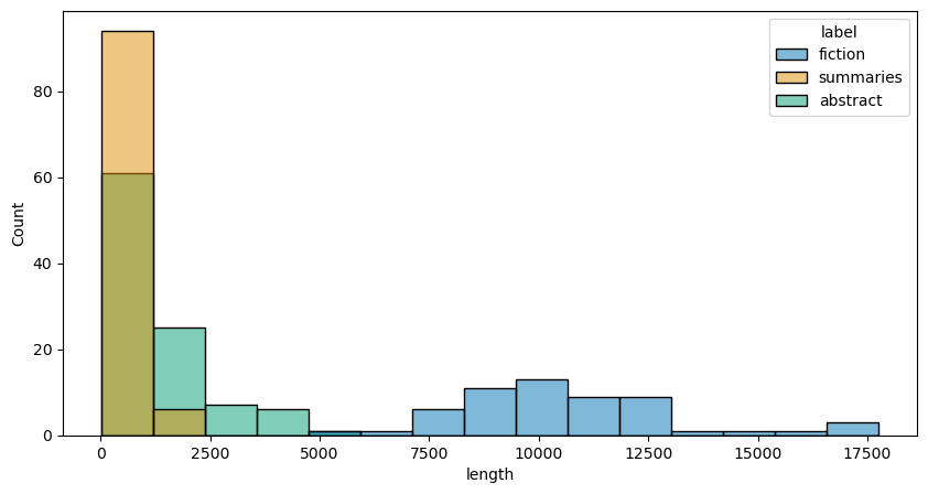
12.3.2. Document length#
The first of our metrics is a simple one: document length. Document length is a
surprisingly effective indicator of different genres, and, even better, it’s
very easy information to collect. In fact, there’s no need to write custom
code; just use len(). We assign the result to a new column in our manifest.
lengths = [len(doc) for doc in docs]
manifest.loc[:, 'length'] = lengths
histplot(manifest, 'length')
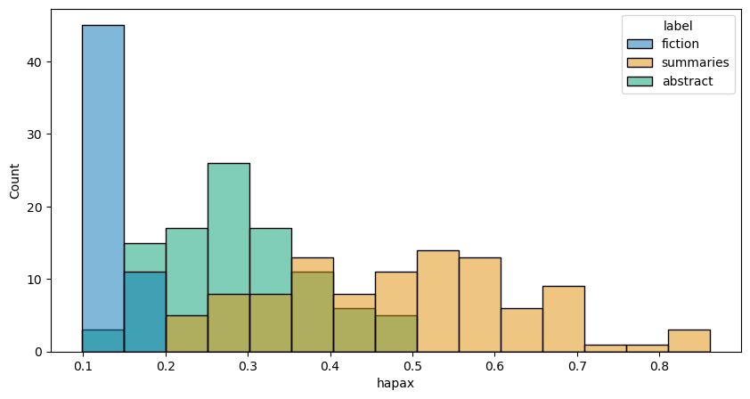
12.3.3. Hapax richness#
Our second metric is hapax richness. If you’ll recall from the second day of our Getting Started with Textual Data workshop series, a hapax (short for “hapax legomenon”) is a word that occurs only once in a document. Researchers, especially those working in authorship attribution, will use such words to create a measure of a document’s lexical complexity: the more hapaxes in a document, the more lexically complex that document is said to be.
Generating a hapax richness metric involves finding all hapaxes in a document. Once we’ve done so, we simply take the sum of those tokens over the total number of tokens in a document.
def hapax_richness(doc):
    """Get the hapax richness for a document."""
    toklist = [tok for tok in doc if tok.is_alpha]
    counts = Counter(tok.text for tok in toklist)
    hapaxes = Counter(tok for tok, count in counts.items() if count == 1)

    return hapaxes.total() / counts.total()

hapaxes = [hapax_richness(doc) for doc in docs]
manifest.loc[:, 'hapax'] = hapaxes
histplot(manifest, 'hapax')
Let’s pause and look at our two metrics with some .groupby() views in
pandas.
Mean distribution of features:
manifest.groupby('label')[['length', 'hapax']].mean()
| length | hapax | |
|---|---|---|
| label | ||
| abstract | 1285.600000 | 0.288841 |
| fiction | 10649.107143 | 0.135776 |
| summaries | 412.910000 | 0.485768 |
Determining whether features are correlated is also useful:
manifest.groupby('label')[['length', 'hapax']].corr()
| length | hapax | ||
|---|---|---|---|
| label | |||
| abstract | length | 1.000000 | -0.502604 |
| hapax | -0.502604 | 1.000000 | |
| fiction | length | 1.000000 | -0.819036 |
| hapax | -0.819036 | 1.000000 | |
| summaries | length | 1.000000 | -0.811724 |
| hapax | -0.811724 | 1.000000 |
It makes sense that length and hapax richness tend to be negatively correlated: the longer a text is, the more likely we are to see repeated words. In this sense, as it stands our hapax feature might not be as representative as we’d like it to be, especially when it comes to a document class like fiction. Surely there are rare, potentially important words in the fiction, but they’re largely blurred by the length of the documents. To mitigate this, we could use a window size to determine hapax richness, modifying the code above, for example, to break texts into smaller chunks and get a mean hapax score for all chunks. We won’t do this now, but keep in mind that you may have to make such modifications when engineering features.
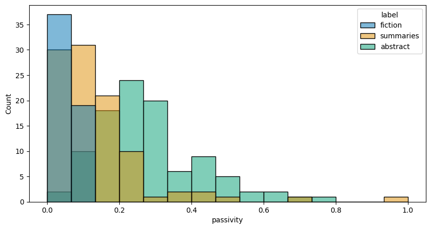
12.3.4. Active and passive voice#
From here, our features will be a little more complex. That complexity is twofold. First, these features require more coding work than the ones above; and second, they require us to think more carefully about relationships across our corpus.
To wit: this next feature concerns the distinction between active and passive
voice. The hypothesis here is that the objective, report-like nature of
abstracts (and perhaps summaries) will have more passive voice overall than in
fiction, which tends to be focused on present action. To measure this, we’ll
use spaCy’s dependency parser to identify the percentage of passive voice
subjects in a document, versus active subjects.
We’ll implement this in a function, which counts the number of passive subjects and the number of active subjects in each sentence of the document. Then, it sums the total number of subjects and divides the number of passive subjects by that total.
def score_passive(doc):
    """Score the passiveness of a document."""
    subj = Counter(passive = 0, active = 0)
    for sent in doc.sents:
        for tok in sent:
            if tok.dep_ in ('nsubj', 'csubj'):
                subj['active'] += 1
            elif tok.dep_ in ('nsubjpass', 'csubjpass'):
                subj['passive'] += 1
            else:
                continue

    return subj['passive'] / subj.total()

passivity = [score_passive(doc) for doc in docs]
manifest.loc[:, 'passivity'] = passivity
histplot(manifest, 'passivity')
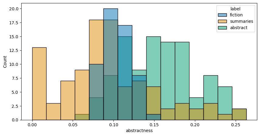
12.3.5. Abstract nouns#
The following code follows a similar structure to the code above. Below, we use
spaCy’s part-of-speech tags to identify nouns in a document. Then we
determine whether these are abstract nouns, on the theory that abstracts and
summaries are likely to have more nouns that denote ideas, qualities,
relationships, etc. than fiction.
But how do we find an abstract noun? One simple way is to consider a noun’s suffix. Suffixes like -acy or -ism (e.g. accuracy, isomorphism) and -hip or -ity (e.g. relationship, fixity) are good, general markers of abstract nouns. They’re not always a perfect match, but they can give us a general sense of what kind of noun it is that we’re working with.
ABSTRACT_SUFFIX = (
    'acy', 'ncy', 'nce', 'ism', 'ity', 'ty', 'ent', 'ess', 'hip', 'ion'
)

def score_abstract(doc):
    """Score the abstractness of a document."""
    nouns = Counter(abstract = 0, not_abstract = 0)
    for tok in doc:
        if not tok.pos_ == 'NOUN':
            continue
        if tok.suffix_ in ABSTRACT_SUFFIX:
            nouns['abstract'] += 1
        else:
            nouns['not_abstract'] += 1

    return nouns['abstract'] / nouns.total()

abstractness = [score_abstract(doc) for doc in docs]
manifest.loc[:, 'abstractness'] = abstractness
histplot(manifest, 'abstractness')
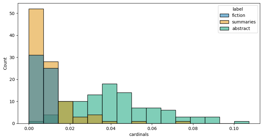
12.3.6. Cardinal numbers#
So far we’ve been eliding potentially important differences between abstracts
and summaries. Let’s develop a metric that might help us distinguish between
the two of them. One such metric could be a simple count of the number of
cardinal numbers in a document: we’d expect summaries to have less than
abstracts (whether because the latter reports various metrics, or because they
often contain citations, dates, etc.). Using spaCy’s part-of-speech tagger
will help us identify these tokens. We count these tokens and divide that
number by the length of the document.
def score_cardinals(doc):
    """Get number of cardinal numbers and normalize on document length."""
    counts = Counter(tok.tag_ for tok in doc if tok.tag_ == 'CD')

    return counts.total() / len(doc)

cardinals = [score_cardinals(doc) for doc in docs]
manifest.loc[:, 'cardinals'] = cardinals
histplot(manifest, 'cardinals')
12.4. Modeling II#
With our features engineered, it’s time to build another model. This time, however, we send it a much smaller set of features, rather than that giant DTM of tf-idf vectors. The workflow is almost entirely the same, save for two changes:
We scale our data and normalize features to a
[0,1]scale.We change the type of distribution our model assumes. A multinomial distribution is the norm for text, as it works well with categorical counts. But we’re no longer working with text data per se; we’re working with data about text, and the values represented therein are continuous. Because of this, we need to use a model that assumes a Gaussian (or normal) distribution.
First, let’s get our features.
feats = ['length', 'hapax', 'passivity', 'abstractness', 'cardinals']
features = manifest[feats].values
Now, we scale them with MinMaxScaler.
minmax = MinMaxScaler()
scaled = minmax.fit_transform(features)
The rest should feel familiar: split the data…
train_data, test_data, train_labels, test_labels = train_test_split(
    scaled,
    manifest['label_int'],
    test_size = 0.3,
    shuffle = True,
    random_state = 357,
)
…and train the model.
model = GaussianNB()
model.fit(train_data, train_labels)
preds = model.predict(test_data)
How did we do?
report = classification_report(test_labels, preds, target_names = target_names)
print(report)
              precision    recall  f1-score   support

     fiction       1.00      1.00      1.00        22
   summaries       0.97      1.00      0.99        33
    abstract       1.00      0.95      0.98        22

    accuracy                           0.99        77
   macro avg       0.99      0.98      0.99        77
weighted avg       0.99      0.99      0.99        77
Surprisingly well, actually! In fact, this second model is arguably better than the first one we built. It’s probably still overfitted to fiction, but the scores for the other document classes indicate that it’s been able to generalize out from specific words to a broader class of features that typify one kind of document from the next. And – just as important – it’s been able to do so with a far smaller set of features. Whereas the DTM we used to train the first model had ~18.5k features, this one only needs five.