13. Word Embeddings#
Our sessions so far have worked off the idea of document annotation to produce metadata about texts. We’ve used this information for everything from information retrieval tasks (Chapter 2) to predictive classification (Chapter 3). Along the way, we’ve also made some passing discussions about how such annotations work to quantify or identify the semantics of those tasks (our work with POS tags, for example). But what we haven’t yet done is produce a model of semantic meaning ourselves. This is another core task of NLP, and there are several different ways to approach building a statistical representation of tokens’ meanings. The present chapter discusses one of the most popular methods of doing so: word embeddings. Below, we’ll overview what word embeddings are, demonstrate how to build and use them, talk about important considerations regarding bias, and apply all this to a document clustering task.
The corpus we’ll use is Melanie Walsh’s collection of ~380 obituaries from the New York Times. If you participated in our Getting Started with Textual Data series, you’ll be familiar with this corpus: we used it in the context of tf-idf scores. Our return to it here is meant to chime with that discussion, for word embeddings enable us to perform a similar kind of text vectorization. Though, as we’ll discuss, the resultant vectors will be considerably more feature-rich than what we could achieve with tf-idf alone.
Learning objectives
By the end of this chapter, you will be able to:
Explain what word embeddings are
Use
gensimto train and load word embeddings modelsIdentify and analyze word relationships in these models
Recognize how bias can inhere in embeddings
Encode documents with a word embeddings model
13.1. How It Works#
Prior to the advent of Transformer models, word embedding served as a state-of-the-art technique for representing semantic relationships between tokens. The technique was first introduced in 2013, and it spawned a host of different variants that completely flooded the field of NLP until about 2018. In part, word embedding’s popularity stems from the relatively simple intuition behind it, which is known as the distributional hypothesis: “you shall know a word by the company it keeps!” (J.R. Firth). Words that appear in similar contexts, in other words, have similar meanings, and what word embeddings do is represent that context-specific information through a set of features. As a result, similar words share similar data representations, and we can leverage that similarity to explore the semantic space of a corpus, to encode documents with feature-rich data, and more.
If you’re familiar with tf-idf vectors, the underlying data structure of word embeddings is the same: every word is represented by a vector of features. But a key difference lies in the sparsity of the vectors – or, in the case of word embeddings, the lack of sparsity. As we saw in the last chapter, tf-idf vectors can suffer from the curse of dimensionality, something that’s compounded by the fact that such vectors must contain features for every word in corpus, regardless of whether a document has that word. This means tf-idf vectors are highly sparse: they contain many 0s. Word embeddings, on the other hand, do not. They’re what we call dense representations. Each one is a fixed-length, non-sparse vector (of 50-300 dimensions, usually) that is much more information-rich than tf-idf. As a result, embeddings tend to be capable of representing more nuanced relationships between corpus words – a performance improvement that is further boosted by the fact that many of the most popular models had the advantage of being trained on billions and billions of tokens.
The other major difference between these vectors and tf-idf lies in how the former are created. While at root, word embeddings represent token co-occurrence data (just like a document-term matrix), they are the product of millions of guesses made by a neural network. Training this network involves making predictions about a target word, based on that word’s context. We are not going to delve into the math behind these predictions (though this post does); however, it is worth noting that there are two different training set ups for a word embedding model:
Common Bag of Words (CBOW): given a window of words on either side of a target, the network tries to predict what word the target should be
Skip-grams: the network starts with the word in the middle of a window and picks random words within this window to use as its prediction targets
As you may have noticed, these are just mirrored versions of one another. CBOW starts from context, while skip-gram tries to rebuild context. Regardless, in both cases the network attempts to maximize the likelihood of its predictions, updating its weights accordingly over the course of training. Words that repeatedly appear in similar contexts will help shape thse weights, and in turn the model will associate such words with similar vector representations. If you’d like to see all this in action, Xin Rong has produced a fantastic interactive visualization of how word embedding models learn.
Of course, the other way to understand how word embeddings work is to use them yourself. We’ll move on to doing so now.
13.2. Preliminaries#
Here are the libraries we will use in this chapter.
from pathlib import Path
from collections import Counter
from tabulate import tabulate
import numpy as np
import pandas as pd
from gensim.models import KeyedVectors
from sklearn.manifold import TSNE
from sklearn.cluster import AgglomerativeClustering
import matplotlib.pyplot as plt
import seaborn as sns
We also initialize an input directory and load a file manifest.
indir = Path("data/section_two/s3")

manifest = pd.read_csv(indir.joinpath("manifest.csv"), index_col = 0)
manifest.info()
<class 'pandas.core.frame.DataFrame'>
Index: 379 entries, 0 to 378
Data columns (total 3 columns):
 #   Column     Non-Null Count  Dtype
---  ------     --------------  -----
 0   name       379 non-null    object
 1   year       379 non-null    int64
 2   file_name  379 non-null    object
dtypes: int64(1), object(2)
memory usage: 11.8+ KB
And finally we’ll load the obituaries. While the past two sessions have required full-text representations of documents, word embeddings work best with bags of words, especially when it comes to doing analysis with them. Accordingly, each of the files in the corpus have already processed by a text cleaning pipeline: they represent the lowercase, stopped, and lemmatized versions of the originals.
corpus = []
for fname in manifest['file_name']:
    with indir.joinpath(f"obits/{fname}").open('r') as fin:
        doc = fin.read()
        corpus.append(doc.split())
With this time, it’s time to move to the model.
13.3. Using an Embeddings Model#
At this point, we are at a crossroads. On the one hand, we could train a word
embeddings model using our corpus documents as is. The gensim library offers
functionality for this, and it’s a relatively easy operation. On the other, we
could use pre-made embeddings, which are usually trained on a more general –
and much larger – set of documents. There is a trade-off here:
Training a corpus-specific model will more faithfully represent the token behavior of the texts we’d like to analyze, but these representations could be too specific, especially if the model doesn’t have enough data to train on; the resultant embeddings may be closer to topic models than to word-level semantics
Using pre-made embeddings gives us the benefit of generalization: the vectors will cleave more closely to how we understand language; but such embeddings might a) miss out on certain nuances we’d like to capture, or b) introduce biases into our corpus (more on this below)
In our case, the decision is difficult. When preparing this reader, we (Tyler and Carl) found that a model trained on the obituaries alone did not produce vectors that could fully demonstrate the capabilities of the word embedding technique. The corpus is just a little too specific, and perhaps a little too small. We could’ve used a larger corpus, but doing so would introduce slow-downs in the workshop session. Because of this, we’ve gone with a pre-made model: the Stanford GloVe embeddings (the 200-dimension version). GloVe was trained on billions of tokens, spanning Wikipedia data, newswire articles, even Twitter. More, the model’s developers offer several different dimension sizes, which are helpful for selecting embeddings with the right amount of detail.
That said, going with GloVe introduces its own problems. For one thing, we can’t show you how to train a word embeddings model itself – at least not live. The code to do so, however, is reproduced below:
from gensim.models import Word2Vec

n_dimensions = 100
model = Word2Vec(n_dimensions)
model.build_vocab(corpus)
model.train(corpus, total_words = model.corpus_total_words, epochs = 5)
Another problem has to do with the data GloVe was trained on. It’s so large that we can’t account for all the content, and this becomes particularly detrimental when it comes to bias. Researchers have found that general embeddings models reproduce gender-discriminatory language, even hate speech, by virtue of the fact that they are trained on huge amounts of text data, often without consideration of whether the content of such data is something one would endorse. GloVe is known to be biased in this way. We’ll show an example later on in this chapter and will discuss this in much more detail during our live session, but for now just note that the effects of bias do shape how we represent our corpus, and it’s important to keep an eye out for this when working with the data.
13.3.1. Loading a model#
With all that said, we can move on. Below, we load GloVe embeddings into our
workspace using a gensim wrapper.
model_path = indir.joinpath("glove/glove-wiki-gigaword_200d.bin")
model = KeyedVectors.load(model_path.as_posix())
The KeyedVectors object acts much like a Python dictionary, and you can do
certain Python operations directly on it.
print("Number of tokens in the model:", len(model))
Number of tokens in the model: 400000
13.3.2. Token mappings#
Each token in the model has an associated index. This mapping is accessible via
.key_to_index.
model.key_to_index
{'the': 0,
 ',': 1,
 '.': 2,
 'of': 3,
 'to': 4,
 'and': 5,
 'in': 6,
 'a': 7,
 '"': 8,
 "'s": 9,
 'for': 10,
 '-': 11,
 'that': 12,
 'on': 13,
 'is': 14,
 'was': 15,
 'said': 16,
 'with': 17,
 'he': 18,
 'as': 19,
 'it': 20,
 'by': 21,
 'at': 22,
 '(': 23,
 ')': 24,
 'from': 25,
 'his': 26,
 "''": 27,
 '``': 28,
 'an': 29,
 'be': 30,
 'has': 31,
 'are': 32,
 'have': 33,
 'but': 34,
 'were': 35,
 'not': 36,
 'this': 37,
 'who': 38,
 'they': 39,
 'had': 40,
 'i': 41,
 'which': 42,
 'will': 43,
 'their': 44,
 ':': 45,
 'or': 46,
 'its': 47,
 'one': 48,
 'after': 49,
 'new': 50,
 'been': 51,
 'also': 52,
 'we': 53,
 'would': 54,
 'two': 55,
 'more': 56,
 "'": 57,
 'first': 58,
 'about': 59,
 'up': 60,
 'when': 61,
 'year': 62,
 'there': 63,
 'all': 64,
 '--': 65,
 'out': 66,
 'she': 67,
 'other': 68,
 'people': 69,
 "n't": 70,
 'her': 71,
 'percent': 72,
 'than': 73,
 'over': 74,
 'into': 75,
 'last': 76,
 'some': 77,
 'government': 78,
 'time': 79,
 '$': 80,
 'you': 81,
 'years': 82,
 'if': 83,
 'no': 84,
 'world': 85,
 'can': 86,
 'three': 87,
 'do': 88,
 ';': 89,
 'president': 90,
 'only': 91,
 'state': 92,
 'million': 93,
 'could': 94,
 'us': 95,
 'most': 96,
 '_': 97,
 'against': 98,
 'u.s.': 99,
 'so': 100,
 'them': 101,
 'what': 102,
 'him': 103,
 'united': 104,
 'during': 105,
 'before': 106,
 'may': 107,
 'since': 108,
 'many': 109,
 'while': 110,
 'where': 111,
 'states': 112,
 'because': 113,
 'now': 114,
 'city': 115,
 'made': 116,
 'like': 117,
 'between': 118,
 'did': 119,
 'just': 120,
 'national': 121,
 'day': 122,
 'country': 123,
 'under': 124,
 'such': 125,
 'second': 126,
 'then': 127,
 'company': 128,
 'group': 129,
 'any': 130,
 'through': 131,
 'china': 132,
 'four': 133,
 'being': 134,
 'down': 135,
 'war': 136,
 'back': 137,
 'off': 138,
 'south': 139,
 'american': 140,
 'minister': 141,
 'police': 142,
 'well': 143,
 'including': 144,
 'team': 145,
 'international': 146,
 'week': 147,
 'officials': 148,
 'still': 149,
 'both': 150,
 'even': 151,
 'high': 152,
 'part': 153,
 'told': 154,
 'those': 155,
 'end': 156,
 'former': 157,
 'these': 158,
 'make': 159,
 'billion': 160,
 'work': 161,
 'our': 162,
 'home': 163,
 'school': 164,
 'party': 165,
 'house': 166,
 'old': 167,
 'later': 168,
 'get': 169,
 'another': 170,
 'tuesday': 171,
 'news': 172,
 'long': 173,
 'five': 174,
 'called': 175,
 '1': 176,
 'wednesday': 177,
 'military': 178,
 'way': 179,
 'used': 180,
 'much': 181,
 'next': 182,
 'monday': 183,
 'thursday': 184,
 'friday': 185,
 'game': 186,
 'here': 187,
 '?': 188,
 'should': 189,
 'take': 190,
 'very': 191,
 'my': 192,
 'north': 193,
 'security': 194,
 'season': 195,
 'york': 196,
 'how': 197,
 'public': 198,
 'early': 199,
 'according': 200,
 'several': 201,
 'court': 202,
 'say': 203,
 'around': 204,
 'foreign': 205,
 '10': 206,
 'until': 207,
 'set': 208,
 'political': 209,
 'says': 210,
 'market': 211,
 'however': 212,
 'family': 213,
 'life': 214,
 'same': 215,
 'general': 216,
 '–': 217,
 'left': 218,
 'good': 219,
 'top': 220,
 'university': 221,
 'going': 222,
 'number': 223,
 'major': 224,
 'known': 225,
 'points': 226,
 'won': 227,
 'six': 228,
 'month': 229,
 'dollars': 230,
 'bank': 231,
 '2': 232,
 'iraq': 233,
 'use': 234,
 'members': 235,
 'each': 236,
 'area': 237,
 'found': 238,
 'official': 239,
 'sunday': 240,
 'place': 241,
 'go': 242,
 'based': 243,
 'among': 244,
 'third': 245,
 'times': 246,
 'took': 247,
 'right': 248,
 'days': 249,
 'local': 250,
 'economic': 251,
 'countries': 252,
 'see': 253,
 'best': 254,
 'report': 255,
 'killed': 256,
 'held': 257,
 'business': 258,
 'west': 259,
 'does': 260,
 'own': 261,
 '%': 262,
 'came': 263,
 'law': 264,
 'months': 265,
 'women': 266,
 "'re": 267,
 'power': 268,
 'think': 269,
 'service': 270,
 'children': 271,
 'bush': 272,
 'show': 273,
 '/': 274,
 'help': 275,
 'chief': 276,
 'saturday': 277,
 'system': 278,
 'john': 279,
 'support': 280,
 'series': 281,
 'play': 282,
 'office': 283,
 'following': 284,
 'me': 285,
 'meeting': 286,
 'expected': 287,
 'late': 288,
 'washington': 289,
 'games': 290,
 'european': 291,
 'league': 292,
 'reported': 293,
 'final': 294,
 'added': 295,
 'without': 296,
 'british': 297,
 'white': 298,
 'history': 299,
 'man': 300,
 'men': 301,
 'became': 302,
 'want': 303,
 'march': 304,
 'case': 305,
 'few': 306,
 'run': 307,
 'money': 308,
 'began': 309,
 'open': 310,
 'name': 311,
 'trade': 312,
 'center': 313,
 '3': 314,
 'israel': 315,
 'oil': 316,
 'too': 317,
 'al': 318,
 'film': 319,
 'win': 320,
 'led': 321,
 'east': 322,
 'central': 323,
 '20': 324,
 'air': 325,
 'come': 326,
 'chinese': 327,
 'town': 328,
 'leader': 329,
 'army': 330,
 'line': 331,
 'never': 332,
 'little': 333,
 'played': 334,
 'prime': 335,
 'death': 336,
 'companies': 337,
 'least': 338,
 'put': 339,
 'forces': 340,
 'past': 341,
 'de': 342,
 'half': 343,
 'june': 344,
 'saying': 345,
 'know': 346,
 'federal': 347,
 'french': 348,
 'peace': 349,
 'earlier': 350,
 'capital': 351,
 'force': 352,
 'great': 353,
 'union': 354,
 'near': 355,
 'released': 356,
 'small': 357,
 'department': 358,
 'every': 359,
 'health': 360,
 'japan': 361,
 'head': 362,
 'ago': 363,
 'night': 364,
 'big': 365,
 'cup': 366,
 'election': 367,
 'region': 368,
 'director': 369,
 'talks': 370,
 'program': 371,
 'far': 372,
 'today': 373,
 'statement': 374,
 'july': 375,
 'although': 376,
 'district': 377,
 'again': 378,
 'born': 379,
 'development': 380,
 'leaders': 381,
 'council': 382,
 'close': 383,
 'record': 384,
 'along': 385,
 'county': 386,
 'france': 387,
 'went': 388,
 'point': 389,
 'must': 390,
 'spokesman': 391,
 'your': 392,
 'member': 393,
 'plan': 394,
 'financial': 395,
 'april': 396,
 'recent': 397,
 'campaign': 398,
 'become': 399,
 'troops': 400,
 'whether': 401,
 'lost': 402,
 'music': 403,
 '15': 404,
 'got': 405,
 'israeli': 406,
 '30': 407,
 'need': 408,
 '4': 409,
 'lead': 410,
 'already': 411,
 'russia': 412,
 'though': 413,
 'might': 414,
 'free': 415,
 'hit': 416,
 'rights': 417,
 '11': 418,
 'information': 419,
 'away': 420,
 '12': 421,
 '5': 422,
 'others': 423,
 'control': 424,
 'within': 425,
 'large': 426,
 'economy': 427,
 'press': 428,
 'agency': 429,
 'water': 430,
 'died': 431,
 'career': 432,
 'making': 433,
 '...': 434,
 'deal': 435,
 'attack': 436,
 'side': 437,
 'seven': 438,
 'better': 439,
 'less': 440,
 'september': 441,
 'once': 442,
 'clinton': 443,
 'main': 444,
 'due': 445,
 'committee': 446,
 'building': 447,
 'conference': 448,
 'club': 449,
 'january': 450,
 'decision': 451,
 'stock': 452,
 'america': 453,
 'given': 454,
 'give': 455,
 'often': 456,
 'announced': 457,
 'television': 458,
 'industry': 459,
 'order': 460,
 'young': 461,
 "'ve": 462,
 'palestinian': 463,
 'age': 464,
 'start': 465,
 'administration': 466,
 'russian': 467,
 'prices': 468,
 'round': 469,
 'december': 470,
 'nations': 471,
 "'m": 472,
 'human': 473,
 'india': 474,
 'defense': 475,
 'asked': 476,
 'total': 477,
 'october': 478,
 'players': 479,
 'bill': 480,
 'important': 481,
 'southern': 482,
 'move': 483,
 'fire': 484,
 'population': 485,
 'rose': 486,
 'november': 487,
 'include': 488,
 'further': 489,
 'nuclear': 490,
 'street': 491,
 'taken': 492,
 'media': 493,
 'different': 494,
 'issue': 495,
 'received': 496,
 'secretary': 497,
 'return': 498,
 'college': 499,
 'working': 500,
 'community': 501,
 'eight': 502,
 'groups': 503,
 'despite': 504,
 'level': 505,
 'largest': 506,
 'whose': 507,
 'attacks': 508,
 'germany': 509,
 'august': 510,
 'change': 511,
 'church': 512,
 'nation': 513,
 'german': 514,
 'station': 515,
 'london': 516,
 'weeks': 517,
 'having': 518,
 '18': 519,
 'research': 520,
 'black': 521,
 'services': 522,
 'story': 523,
 '6': 524,
 'europe': 525,
 'sales': 526,
 'policy': 527,
 'visit': 528,
 'northern': 529,
 'lot': 530,
 'across': 531,
 'per': 532,
 'current': 533,
 'board': 534,
 'football': 535,
 'ministry': 536,
 'workers': 537,
 'vote': 538,
 'book': 539,
 'fell': 540,
 'seen': 541,
 'role': 542,
 'students': 543,
 'shares': 544,
 'iran': 545,
 'process': 546,
 'agreement': 547,
 'quarter': 548,
 'full': 549,
 'match': 550,
 'started': 551,
 'growth': 552,
 'yet': 553,
 'moved': 554,
 'possible': 555,
 'western': 556,
 'special': 557,
 '100': 558,
 'plans': 559,
 'interest': 560,
 'behind': 561,
 'strong': 562,
 'england': 563,
 'named': 564,
 'food': 565,
 'period': 566,
 'real': 567,
 'authorities': 568,
 'car': 569,
 'term': 570,
 'rate': 571,
 'race': 572,
 'nearly': 573,
 'korea': 574,
 'enough': 575,
 'site': 576,
 'opposition': 577,
 'keep': 578,
 '25': 579,
 'call': 580,
 'future': 581,
 'taking': 582,
 'island': 583,
 '2008': 584,
 '2006': 585,
 'road': 586,
 'outside': 587,
 'really': 588,
 'century': 589,
 'democratic': 590,
 'almost': 591,
 'single': 592,
 'share': 593,
 'leading': 594,
 'trying': 595,
 'find': 596,
 'album': 597,
 'senior': 598,
 'minutes': 599,
 'together': 600,
 'congress': 601,
 'index': 602,
 'australia': 603,
 'results': 604,
 'hard': 605,
 'hours': 606,
 'land': 607,
 'action': 608,
 'higher': 609,
 'field': 610,
 'cut': 611,
 'coach': 612,
 'elections': 613,
 'san': 614,
 'issues': 615,
 'executive': 616,
 'february': 617,
 'production': 618,
 'areas': 619,
 'river': 620,
 'face': 621,
 'using': 622,
 'japanese': 623,
 'province': 624,
 'park': 625,
 'price': 626,
 'commission': 627,
 'california': 628,
 'father': 629,
 'son': 630,
 'education': 631,
 '7': 632,
 'village': 633,
 'energy': 634,
 'shot': 635,
 'short': 636,
 'africa': 637,
 'key': 638,
 'red': 639,
 'association': 640,
 'average': 641,
 'pay': 642,
 'exchange': 643,
 'eu': 644,
 'something': 645,
 'gave': 646,
 'likely': 647,
 'player': 648,
 'george': 649,
 '2007': 650,
 'victory': 651,
 '8': 652,
 'low': 653,
 'things': 654,
 '2010': 655,
 'pakistan': 656,
 '14': 657,
 'post': 658,
 'social': 659,
 'continue': 660,
 'ever': 661,
 'look': 662,
 'chairman': 663,
 'job': 664,
 '2000': 665,
 'soldiers': 666,
 'able': 667,
 'parliament': 668,
 'front': 669,
 'himself': 670,
 'problems': 671,
 'private': 672,
 'lower': 673,
 'list': 674,
 'built': 675,
 '13': 676,
 'efforts': 677,
 'dollar': 678,
 'miles': 679,
 'included': 680,
 'radio': 681,
 'live': 682,
 'form': 683,
 'david': 684,
 'african': 685,
 'increase': 686,
 'reports': 687,
 'sent': 688,
 'fourth': 689,
 'always': 690,
 'king': 691,
 '50': 692,
 'tax': 693,
 'taiwan': 694,
 'britain': 695,
 '16': 696,
 'playing': 697,
 'title': 698,
 'middle': 699,
 'meet': 700,
 'global': 701,
 'wife': 702,
 '2009': 703,
 'position': 704,
 'located': 705,
 'clear': 706,
 'ahead': 707,
 '2004': 708,
 '2005': 709,
 'iraqi': 710,
 'english': 711,
 'result': 712,
 'release': 713,
 'violence': 714,
 'goal': 715,
 'project': 716,
 'closed': 717,
 'border': 718,
 'body': 719,
 'soon': 720,
 'crisis': 721,
 'division': 722,
 '&': 723,
 'served': 724,
 'tour': 725,
 'hospital': 726,
 'kong': 727,
 'test': 728,
 'hong': 729,
 'u.n.': 730,
 'inc.': 731,
 'technology': 732,
 'believe': 733,
 'organization': 734,
 'published': 735,
 'weapons': 736,
 'agreed': 737,
 'why': 738,
 'nine': 739,
 'summer': 740,
 'wanted': 741,
 'republican': 742,
 'act': 743,
 'recently': 744,
 'texas': 745,
 'course': 746,
 'problem': 747,
 'senate': 748,
 'medical': 749,
 'un': 750,
 'done': 751,
 'reached': 752,
 'star': 753,
 'continued': 754,
 'investors': 755,
 'living': 756,
 'care': 757,
 'signed': 758,
 '17': 759,
 'art': 760,
 'provide': 761,
 'worked': 762,
 'presidential': 763,
 'gold': 764,
 'obama': 765,
 'morning': 766,
 'dead': 767,
 'opened': 768,
 "'ll": 769,
 'event': 770,
 'previous': 771,
 'cost': 772,
 'instead': 773,
 'canada': 774,
 'band': 775,
 'teams': 776,
 'daily': 777,
 '2001': 778,
 'available': 779,
 'drug': 780,
 'coming': 781,
 '2003': 782,
 'investment': 783,
 '’s': 784,
 'michael': 785,
 'civil': 786,
 'woman': 787,
 'training': 788,
 'appeared': 789,
 '9': 790,
 'involved': 791,
 'indian': 792,
 'similar': 793,
 'situation': 794,
 '24': 795,
 'los': 796,
 'running': 797,
 'fighting': 798,
 'mark': 799,
 '40': 800,
 'trial': 801,
 'hold': 802,
 'australian': 803,
 'thought': 804,
 '!': 805,
 'study': 806,
 'fall': 807,
 'mother': 808,
 'met': 809,
 'relations': 810,
 'anti': 811,
 '2002': 812,
 'song': 813,
 'popular': 814,
 'base': 815,
 'tv': 816,
 'ground': 817,
 'markets': 818,
 'ii': 819,
 'newspaper': 820,
 'staff': 821,
 'saw': 822,
 'hand': 823,
 'hope': 824,
 'operations': 825,
 'pressure': 826,
 'americans': 827,
 'eastern': 828,
 'st.': 829,
 'legal': 830,
 'asia': 831,
 'budget': 832,
 'returned': 833,
 'considered': 834,
 'love': 835,
 'wrote': 836,
 'stop': 837,
 'fight': 838,
 'currently': 839,
 'charges': 840,
 'try': 841,
 'aid': 842,
 'ended': 843,
 'management': 844,
 'brought': 845,
 'cases': 846,
 'decided': 847,
 'failed': 848,
 'network': 849,
 'works': 850,
 'gas': 851,
 'turned': 852,
 'fact': 853,
 'vice': 854,
 'ca': 855,
 'mexico': 856,
 'trading': 857,
 'especially': 858,
 'reporters': 859,
 'afghanistan': 860,
 'common': 861,
 'looking': 862,
 'space': 863,
 'rates': 864,
 'manager': 865,
 'loss': 866,
 '2011': 867,
 'justice': 868,
 'thousands': 869,
 'james': 870,
 'rather': 871,
 'fund': 872,
 'thing': 873,
 'republic': 874,
 'opening': 875,
 'accused': 876,
 'winning': 877,
 'scored': 878,
 'championship': 879,
 'example': 880,
 'getting': 881,
 'biggest': 882,
 'performance': 883,
 'sports': 884,
 '1998': 885,
 'let': 886,
 'allowed': 887,
 'schools': 888,
 'means': 889,
 'turn': 890,
 'leave': 891,
 'no.': 892,
 'robert': 893,
 'personal': 894,
 'stocks': 895,
 'showed': 896,
 'light': 897,
 'arrested': 898,
 'person': 899,
 'either': 900,
 'offer': 901,
 'majority': 902,
 'battle': 903,
 '19': 904,
 'class': 905,
 'evidence': 906,
 'makes': 907,
 'society': 908,
 'products': 909,
 'regional': 910,
 'needed': 911,
 'stage': 912,
 'am': 913,
 'doing': 914,
 'families': 915,
 'construction': 916,
 'various': 917,
 '1996': 918,
 'sold': 919,
 'independent': 920,
 'kind': 921,
 'airport': 922,
 'paul': 923,
 'judge': 924,
 'internet': 925,
 'movement': 926,
 'room': 927,
 'followed': 928,
 'original': 929,
 'angeles': 930,
 'italy': 931,
 '`': 932,
 'data': 933,
 'comes': 934,
 'parties': 935,
 'nothing': 936,
 'sea': 937,
 'bring': 938,
 '2012': 939,
 'annual': 940,
 'officer': 941,
 'beijing': 942,
 'present': 943,
 'remain': 944,
 'nato': 945,
 '1999': 946,
 '22': 947,
 'remains': 948,
 'allow': 949,
 'florida': 950,
 'computer': 951,
 '21': 952,
 'contract': 953,
 'coast': 954,
 'created': 955,
 'demand': 956,
 'operation': 957,
 'events': 958,
 'islamic': 959,
 'beat': 960,
 'analysts': 961,
 'interview': 962,
 'helped': 963,
 'child': 964,
 'probably': 965,
 'spent': 966,
 'asian': 967,
 'effort': 968,
 'cooperation': 969,
 'shows': 970,
 'calls': 971,
 'investigation': 972,
 'lives': 973,
 'video': 974,
 'yen': 975,
 'runs': 976,
 'tried': 977,
 'bad': 978,
 'described': 979,
 '1994': 980,
 'toward': 981,
 'written': 982,
 'throughout': 983,
 'established': 984,
 'mission': 985,
 'associated': 986,
 'buy': 987,
 'growing': 988,
 'green': 989,
 'forward': 990,
 'competition': 991,
 'poor': 992,
 'latest': 993,
 'banks': 994,
 'question': 995,
 '1997': 996,
 'prison': 997,
 'feel': 998,
 'attention': 999,
 ...}
If you want the vector representation for a token, use either the key or the index.
tok = np.random.choice(model.index_to_key)
idx = model.key_to_index[tok]
print(f"The index position for '{tok}' is {idx}")
The index position for '78th' is 25740
Here’s its vector:
model[idx]
array([-0.14427  , -0.33403  ,  0.45775  , -0.46946  ,  0.32486  ,
       -0.46966  ,  0.27248  , -0.069801 , -0.1452   ,  0.27769  ,
       -0.65446  , -0.13101  , -0.46216  , -0.12218  ,  0.45126  ,
        0.068978 ,  0.26799  , -0.47135  , -0.22237  , -0.05276  ,
       -0.24681  , -0.28646  ,  0.21886  , -0.014155 ,  0.29994  ,
       -0.017748 , -1.1387   ,  0.10395  , -0.13259  , -0.1028   ,
        0.3195   ,  0.67297  , -0.3862   ,  0.15007  , -0.87635  ,
        0.20166  , -0.68379  , -0.31019  ,  0.43356  ,  0.082705 ,
       -0.41499  , -0.26557  ,  0.60204  ,  0.33326  ,  0.31807  ,
        0.68115  ,  0.056629 ,  0.6976   , -0.23515  , -0.5588   ,
        0.11685  ,  0.021157 ,  0.57126  ,  0.49979  , -1.0136   ,
       -0.16494  ,  0.45372  ,  0.40722  , -0.47333  ,  0.019141 ,
       -0.53122  , -0.37901  ,  0.30372  ,  0.40445  ,  0.30727  ,
       -0.041104 , -0.1602   , -0.67757  ,  0.39242  , -0.43911  ,
        0.21599  , -0.055554 ,  0.40778  ,  0.45617  , -0.0956   ,
        0.41711  ,  0.063262 ,  0.35673  , -0.21999  ,  0.32982  ,
        0.084537 , -0.2262   ,  0.64776  ,  0.1196   ,  0.30376  ,
       -0.024766 ,  0.18282  , -0.73633  , -0.31217  ,  0.15465  ,
       -0.27208  , -0.080605 , -0.44106  , -0.27606  ,  0.70544  ,
       -0.12776  , -0.37467  , -0.13289  ,  0.97463  ,  0.023408 ,
       -0.31382  , -0.38444  ,  0.75336  , -0.14982  , -0.39482  ,
       -0.26319  , -0.0028122,  1.0462   ,  0.13512  , -0.56078  ,
        0.083691 , -0.39987  , -0.32548  ,  0.045956 , -0.489    ,
        0.5523   ,  0.031139 , -0.2539   ,  0.38169  , -0.32343  ,
       -1.1613   , -0.47647  ,  0.25196  , -0.15564  , -0.35601  ,
        0.28356  , -0.81928  , -0.014334 , -0.23137  ,  0.22196  ,
       -0.30573  ,  0.079012 ,  0.23627  , -1.1194   , -0.53919  ,
        0.055377 ,  0.28243  ,  0.75231  , -0.24656  ,  0.39558  ,
        0.10234  ,  0.8643   , -0.13513  , -0.61439  , -0.44418  ,
        0.15448  ,  0.033391 ,  0.21326  ,  0.15473  , -0.64362  ,
       -0.006179 ,  0.12181  ,  0.69615  , -0.017563 ,  0.67365  ,
        0.43283  , -0.1154   , -0.23875  , -0.26457  ,  0.29562  ,
       -0.7819   ,  0.24905  , -0.57692  ,  0.12249  ,  0.10244  ,
       -0.059327 , -0.11739  , -0.62648  , -0.34553  , -0.22463  ,
        0.10255  , -0.1263   ,  0.084839 , -0.32339  , -0.20997  ,
        0.69963  , -0.38752  , -0.49736  ,  0.63749  ,  0.11065  ,
        0.25988  , -0.24398  ,  0.099394 ,  0.47701  , -0.59195  ,
       -0.011084 , -0.4131   ,  0.30546  , -0.69945  ,  0.52869  ,
        0.57477  , -0.46084  , -0.49228  , -0.2432   ,  0.0068473,
       -0.19733  ,  0.076383 ,  0.61021  , -0.21718  ,  0.41104  ],
      dtype=float32)
Here are some random tokens in the model:
for tok in np.random.choice(model.index_to_key, 10):
    print(tok)
kedua
ekström
bonder
philometor
karaftu
rrm
subjunctive
furlan
braund
http://www.eurekalert.org
You may find some unexpected tokens in this output. Though it has been ostensibly trained on an English corpus, GloVe contains multilingual text. It also contains lots of noisy tokens, which range from erroneous segmentations (“drummer/percussionist” is one token, for example) to password-like strings and even HTML markup. Depending on your task, you may not notice these tokens, but they do in fact influence the overall shape of the model, and sometimes you’ll find them cropping up when you’re hunting around for similar terms and the like (more on this soon).
13.3.3. Out-of-vocabulary tokens#
While GloVe’s vocabulary sometimes seems too expansive, there are other instances where it’s too restricted.
assert 'unshaped' in model, "Not in vocabulary!"
---------------------------------------------------------------------------
AssertionError                            Traceback (most recent call last)
Cell In[11], line 1
----> 1 assert 'unshaped' in model, "Not in vocabulary!"

AssertionError: Not in vocabulary!
If the model wasn’t trained on a particular word, it won’t have a corresponding vector for that word either. This is crucial. Because models like GloVe only know what they’ve been trained on, you need to be aware of any potential discrepancies between their vocabularies and your corpus data. If you don’t keep this in mind, sending unseen, or out-of-vocabulary, tokens to GloVe will throw errors in your code.
There are a few ways to handle this problem. The most common is to simply not
encode tokens in your corpus that don’t have a corresponding vector in GloVe.
Below, we construct two sets for our corpus data. The first contains all
tokens in the corpus, while the second tracks which of those tokens are in
the model. We identify whether the model has a token using its
.has_index_for() method.
vocab = set(tok for doc in corpus for tok in doc)
in_glove = set(tok for tok in vocab if model.has_index_for(tok))

print("Total words in the corpus vocabulary:", len(vocab))
print("Words not in GloVe:", len(vocab) - len(in_glove))
Total words in the corpus vocabulary: 29330
Words not in GloVe: 1842
Any subsequent code we write will need to reference these sets to determine whether it should encode a token.
While this is what we’ll indeed do below, obviously it isn’t an ideal
situation. But it’s one of the consequences of using premade models. There are,
however, a few other ways to handle out-of-vocabulary terms. Some models offer
special “UNK” tokens, which you could associate with all of your problem
tokens. This, at the very least, enables you to have some representation of
your data. A more complex approach involves taking the mean embedding of the
word vectors surrounding an unknown token; and depending on the model, you can
also train it further, adding extra tokens from your domain-specific text.
Instructions for this last option are available here in the gensim
documentation.
13.4. Word Relationships#
Later on we’ll use GloVe to encode our corpus texts. But before we do, it’s worth demonstrating more generally some of the properties of word vectors. Vector representations of text allow us to perform various mathematical operations on our corpus that approximate semantics. The most common among these operations is finding the cosine similarity between two vectors. Our Getting Started with Textual Data series has a whole chapter on this measure, so if you haven’t encountered it before, we recommend you read that. But in short: cosine similarity measures the difference between vectors’ orientation in a feature space (here, the feature space is comprised of each of the vectors’ 200 dimensions). The closer two vectors are, the more likely they are to share semantic similarities.
13.4.1. Similar tokens#
gensim provides easy access to this measure and other such vector space
operations. To find the cosine similarity between the vectors for two words in
GloVe, simply use the model’s .similarity() method:
a, b = 'calculate', 'compute'
print(f"Similarity of '{a}' and '{b}': {model.similarity(a, b):0.2f}")
Similarity of 'calculate' and 'compute': 0.70
The only difference between the score above and the one that you might produce,
say, with scikit-learn’s cosine similarity implementation is that gensim
bounds its values from [-1,1], whereas the latter uses a [0,1] scale. While
in gensim it’s still the case that similar words score closer to 1, highly
dissimilar words will be closer to -1.
At any rate, we can get the top n most similar words for a word using
.most_similar(). The function defaults to 10 entries, but you can change that
with the topn parameter. We’ll wrap this in a custom function, since we’ll
call it a number of times.
def show_most_similar(*args, func = model.most_similar, **kwargs):
    """Print cosine similarities."""
    similarities = func(*args, **kwargs)
    print(tabulate(similarities, ['Word', 'Score']))
Now we sample some tokens and find their most similar tokens.
targets = np.random.choice(model.index_to_key, 5)
for tok in targets:
    print(f"Tokens most similar to '{tok}'\n")
    show_most_similar(tok)
    print("\n")
Tokens most similar to '1,145'

Word       Score
------  --------
1,153   0.654589
1,165   0.64991
1,155   0.649251
1,085   0.646486
1,535   0.64473
1,089   0.642814
1,062   0.639672
1,761   0.638582
1,027   0.638248
1,293   0.636172


Tokens most similar to 'leterrier'

Word          Score
---------  --------
jouvet     0.614746
calhern    0.603718
couturat   0.583861
feuillade  0.553632
garrel     0.546433
delluc     0.532536
daquin     0.531879
jadot      0.523224
baraguey   0.518989
caprioli   0.517034


Tokens most similar to 'dimech'

Word           Score
----------  --------
benward     0.564739
joeckel     0.548858
axtell      0.531581
triandos    0.529778
pomersbach  0.529727
bambridge   0.52873
kuechly     0.527648
schenn      0.525584
manget      0.518051
appling     0.515033


Tokens most similar to 'manh'

Word       Score
------  --------
luong   0.674575
duc     0.671491
nong    0.621578
phieu   0.621281
nguyen  0.617178
khai    0.586266
muoi    0.570609
cpv     0.563588
tran    0.558068
cuong   0.556909


Tokens most similar to 'elrod'
Word              Score
-------------  --------
hendricks      0.578068
ruskell        0.444554
beason         0.437564
grgurich       0.431078
leuer          0.425855
orimi          0.42451
zarni          0.422594
brooke-taylor  0.421716
fedewa         0.420495
ramsdell       0.418061
It’s also possible to find the least similar word. This is useful to show, because it pressures our idea of what counts as similarity. Mathematical similarity does not always align with concepts like synonyms and antonyms. For example, it’s probably safe to say that the semantic opposite of “good” – that is, its antonym – is “evil.” But in the world of vector spaces, the least similar word to “good” is:
model.most_similar('good', topn = len(model))[-1]
('cw96', -0.6553234457969666)
Just noise! Relatively speaking, the vectors for “good” and “evil” are actually quite similar.
a, b = 'good', 'evil'
print(f"Similarity of '{a}' and '{b}': {model.similarity(a, b):0.2f}")
Similarity of 'good' and 'evil': 0.34
How do we make sense of this? Well, it has to do with the way the word embeddings are created. Since embeddings models are ultimately trained on co-occurrence data, words that tend to appear in similar kinds of contexts will be more similar in a mathematical sense than those that don’t.
Keeping this in mind is also important for considerations of bias. Since, in one sense, embeddings reflect the interchangeability between tokens, they will reinforce negative, even harmful patterns in the data (which is to say in culture at large). For example, consider the most similar words for “doctor” and “nurse.” The latter is locked up within gendered language: according to GloVe, a nurse is like a midwife is like a mother.
for tok in ('doctor', 'nurse'):
    print(f"Tokens most similar to '{tok}'\n")
    show_most_similar(tok)
    print("\n")
Tokens most similar to 'doctor'

Word             Score
------------  --------
physician     0.736021
doctors       0.672406
surgeon       0.655147
dr.           0.652498
nurse         0.651449
medical       0.648189
hospital      0.63638
patient       0.619159
dentist       0.584747
psychiatrist  0.568571


Tokens most similar to 'nurse'

Word            Score
-----------  --------
nurses       0.714051
doctor       0.651449
nursing      0.626937
midwife      0.614592
anesthetist  0.610603
physician    0.610359
hospital     0.609222
mother       0.586503
therapist    0.580488
dentist      0.573556
13.4.2. Concept modeling#
Beyond cosine similarity, there are other word relationships to explore via
vector space math. For example, one way of modeling something like a concept
is to think about what other concepts comprise it. In other words: what plus
what creates a new concept? Could we identify concepts by adding together
vectors to create a new vector? Which words would this new vector be closest to
in the vector space? Using the .similar_by_vector() method, we can find out.
concepts = {
    'beach': ('sand', 'ocean'),
    'hotel': ('vacation', 'room'),
    'airplane': ('air', 'car')
}
for concept in concepts:
    a, b = concepts[concept]
    vector = model[a] + model[b]
    print(f"Tokens most similar to '{a}' + '{b}' (for '{concept}')\n")
    show_most_similar(vector, func = model.similar_by_vector)
    print("\n")
Tokens most similar to 'sand' + 'ocean' (for 'beach')

Word        Score
-------  --------
sand     0.845458
ocean    0.845268
sea      0.687682
beaches  0.667521
waters   0.664894
coastal  0.632485
water    0.618701
coast    0.604373
dunes    0.599333
surface  0.597545


Tokens most similar to 'vacation' + 'room' (for 'hotel')

Word          Score
---------  --------
vacation   0.82346
room       0.810719
rooms      0.704233
bedroom    0.658199
hotel      0.647865
dining     0.634925
stay       0.617807
apartment  0.616495
staying    0.615182
home       0.606009


Tokens most similar to 'air' + 'car' (for 'airplane')

Word          Score
---------  --------
air        0.827957
car        0.810086
vehicle    0.719382
cars       0.671697
truck      0.645963
vehicles   0.637166
passenger  0.625993
aircraft   0.62482
jet        0.618584
airplane   0.610345
Not bad! While our target concepts aren’t the most similar words for these synthetic vectors, they’re often in the top-10 most similar results.
13.4.3. Analogies#
Most famously, word embeddings enable quasi-logical reasoning. Though relationships between antonyms and synonyms do not necessarily map to a vector space, certain analogies do – at least under the right circumstances, and with particular training data. The logic here is that we identify a relationship between two words and we subtract one of those words’ vectors from the other. To that new vector we add in a vector for a target word, which forms the analogy. Querying for the word closest to this modified vector should produce a similar relation between the result and the target word as that between the original pair.
Here, we ask: “strong is to stronger what clear is to X?” Ideally, we’d get “clearer.”
show_most_similar(
    func = model.most_similar,
    positive = ['stronger', 'clear'],
    negative = ['strong']
)
Word         Score
--------  --------
easier    0.633451
should    0.630116
clearer   0.62185
better    0.602637
must      0.601793
need      0.595918
meant     0.594797
harder    0.591297
anything  0.589579
nothing   0.589187
“Paris is to France what Berlin is to X?” Answer: “Germany.”
show_most_similar(
    func = model.most_similar,
    positive = ['france', 'berlin'],
    negative = ['paris']
)
Word        Score
-------  --------
germany  0.835242
german   0.68448
austria  0.612803
poland   0.581331
germans  0.574868
munich   0.543591
belgium  0.532413
britain  0.529541
europe   0.524402
czech    0.515241
Both of the above produce compelling results, though your mileage may vary. Consider the following: “arm is to hand what leg is to X?” We’d expect “foot.”
show_most_similar(
    func = model.most_similar,
    positive = ['hand', 'leg'],
    negative = ['arm']
)
Word         Score
--------  --------
final     0.543408
table     0.540411
legs      0.527352
back      0.523477
saturday  0.522487
round     0.51625
draw      0.516066
second    0.5109
place     0.509784
side      0.508683
Importantly, these results are always going to be specific to the data on which a model was trained. Claims made on the basis of word embeddings that aspire to general linguistic truths would be treading on shaky ground here.
13.5. Document Similarity#
While the above word relationships are relatively abstract (and any such findings therefrom should be couched accordingly), we can ground them with a concrete task. In this final section, we use GloVe embeddings to encode our corpus documents. This involves associating a word vector for each token in an obituary. Of course, GloVe has not been trained on the obituaries, so there may be important differences in token behavior between that model and the corpus; but we can assume that the general nature of GloVe will give us a decent sense of the overall feature space of the corpus. The result will be an enriched representation of each document, the nuances of which may better help us identify things like similarities between obituaries in our corpus.
The other consideration for using GloVe with our specific corpus concerns the
out-of-vocabulary words we’ve already discussed. Before we can encode our
documents, we need to filter out tokens for which GloVe has no representation.
We can do so by referencing the in_glove set we produced above.
pruned = []
for doc in corpus:
    keep = [tok for tok in doc if tok in in_glove]
    pruned.append(keep)
13.5.1. Encoding#
Time to encode. This is an easy operation. All we need to do is run the list of
document’s tokens directly into the model object and gensim will encode each
accordingly. The result will be an (n, 200) array, where n is the number of
tokens we passed to the model; each one will have 200 dimensions.
But if we kept this array as is, we’d run into trouble. Matrix operations often require identically shaped representations, so documents with different lengths would be incomparable. To get around this, we take the mean of all the vectors in a document. The result is a 200-dimension vector that stands as a general representation of a document.
embeddings = [np.mean(model[doc], axis = 0) for doc in pruned]
embeddings = np.array(embeddings)
Let’s quickly check our work.
print("Shape of an encoded document:", model[pruned[0]].shape)
print("Shape of a document vectour:", embeddings[0].shape)
Shape of an encoded document: (485, 200)
Shape of a document vectour: (200,)
13.5.2. Visualizing#
From here, we can use these embeddings for any task that requires feature vectors. For example, let’s plot our documents using t-SNE. First, we reduce the embeddings.
reducer = TSNE(
    n_components = 2,
    learning_rate = 'auto',
    init = 'random',
    random_state = 357,
    n_jobs = -1
)
reduced = reducer.fit_transform(embeddings)
vis = pd.DataFrame({'x': reduced[:,0], 'y': reduced[:,1], 'label': manifest['name']})
Now we define a function to make our plot. We’ll add some people to look for along as well (in this case, a few baseball players)
def sim_plot(data, hue = None, labels = None, n_colors = 3):
    """Create a scatterplot and optionally color/label its points."""
    fig, ax = plt.subplots(figsize = (10, 10))
    pal = sns.color_palette('colorblind', n_colors = n_colors) if hue else None
    g = sns.scatterplot(
        x = 'x', y = 'y',
        hue = hue, palette = pal, alpha = 0.8,
        data = data, ax = ax
    )
    g.set(xticks = [], yticks = [], xlabel = 'Dim. 1', ylabel = 'Dim. 2')

    if labels:
        to_label = data[data['label'].isin(labels)]
        to_label[['x', 'y', 'label']].apply(lambda x: g.text(*x), axis = 1)

    plt.show()

people = ('Jackie Robinson', 'Lou Gehrig', 'Cy Young')
sim_plot(vis, labels = people)
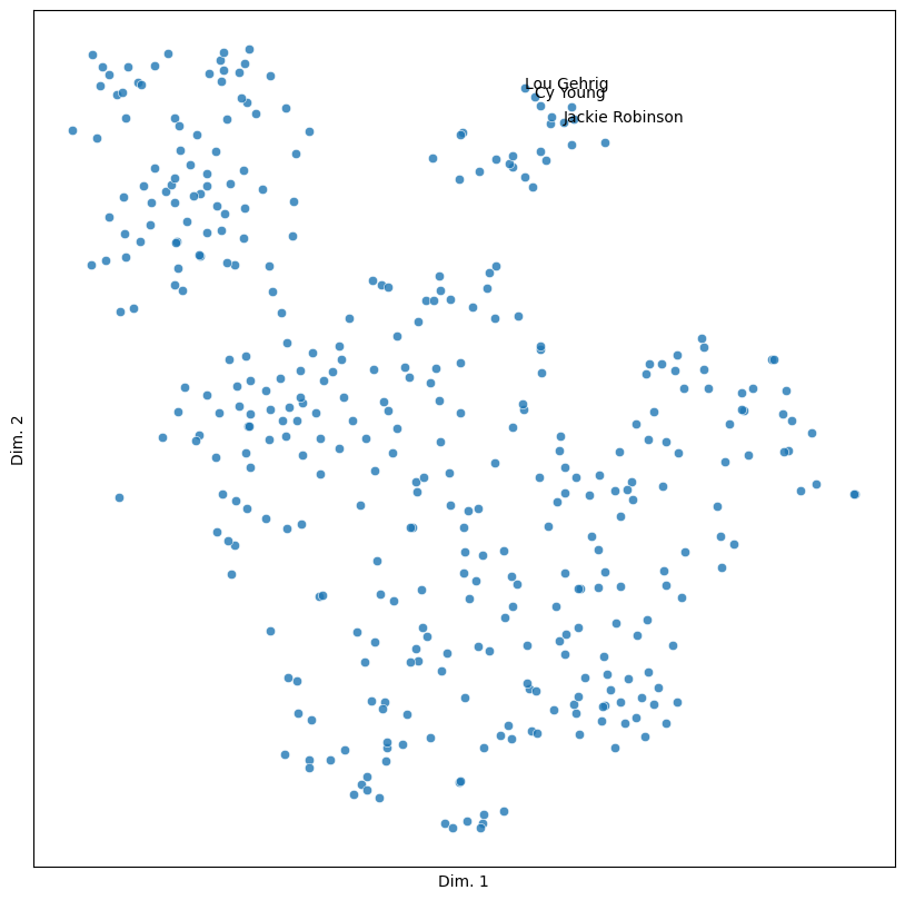
13.5.3. Clustering#
The document embeddings seem to be partitioned into different clusters. We’ll
end by using a hierarchical clusterer to see if we can further specify these
clusters. This involves using the AgglomerativeClustering object, which we
fit to our embeddings. Hierarchical clustering requires a pre-defined number of
clusters. In this case, we use 18.
agg = AgglomerativeClustering(n_clusters = 18)
agg.fit(embeddings)
AgglomerativeClustering(n_clusters=18)In a Jupyter environment, please rerun this cell to show the HTML representation or trust the notebook.
On GitHub, the HTML representation is unable to render, please try loading this page with nbviewer.org.
AgglomerativeClustering(n_clusters=18)
Now we assign the clusterer’s predicted labels to the visualization data DataFrame and re-plot the results.
vis.loc[:, 'cluster'] = agg.labels_
sim_plot(vis, hue = 'cluster', n_colors = 18)
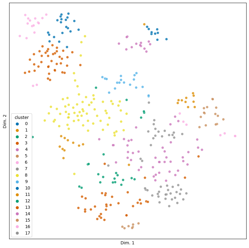
These clusters seem to be both detailed and nicely partitioned, bracketing off, for example, classical musicians and composers (cluster 6) from jazz and popular musicians (cluster 10).
for k in (6, 10):
    people = vis.loc[vis['cluster'] == k, 'label']
    print("Cluster:", k, "\n")
    for person in people:
        print(person)
    print("\n")
Cluster: 6

Maurice Ravel
Constantin Stanislavsky
Bela Bartok
Sergei Eisenstein
Igor Stravinsky
Otto Klemperer
Maria Callas
Arthur Fiedler
Arthur Rubinstein
Andres Segovie
Vladimir Horowitz
Leonard Bernstein
Martha Graham
John Cage
Carlos Montoya
Galina Ulanova


Cluster: 10

Jerome Kern
W C Handy
Billie Holiday
Cole Porter
Coleman Hawkins
Judy Garland
Louis Armstrong
Mahalia Jackson
Stan Kenton
Richard Rodgers
Thelonious Monk
Earl Hines
Muddy Waters
Ethel Merman
Count Basie
Benny Goodman
Miles Davis
Dizzy Gillespie
Gene Kelly
Frank Sinatra
Consider further cluster 5, which seems to be about famous scientists.
for person in vis.loc[vis['cluster'] == 5, 'label']:
    print(person)
Martian Theory
Marie Curie
Elmer Sperry
George E Hale
C E M Clung
Max Planck
A J Dempster
Enrico Fermi
Ross G Harrison
Beno Gutenberg
J Robert Oppenheimer
Jacques Monod
William B Shockley
Linus C Pauling
Carl Sagan
There are, however, some interestingly noisy clusters, like cluster 12. With people like Queen Victoria and William McKinley in this cluster, it at first appears to be about national leaders of various sorts, but the inclusion of others like Al Capone (the gangster) and Ernie Pyle (a journalist) complicate this. If you take a closer look, what really seems to be tying these obituaries together is war. Nearly everyone here was involved in war in some fashion or another – save for Capone, whose inclusion makes for strange bedfellows.
for person in vis.loc[vis['cluster'] == 12, 'label']:
    print(person)
Robert E Lee
Bedford Forrest
Ulysses Grant
William McKinley
Queen Victoria
Geronimo
John P Holland
Alfred Thayer Mahan
Ernie Pyle
George Patton
Al Capone
John Pershing
Douglas MacArthur
Chester Nimitz
Florence Blanchfield
The Duke of Windsor
Depending on your task, these detailed distinctions may not be so desirable. But for us, the document embeddings provide a wonderfully nuanced view of the kinds of people in the obituaries. From here, further exploration might involve focusing on misfits and outliers. Why, for example, is Capone in cluster 12? Or why is Lou Gehrig all by himself in his own cluster? Of course, we could always re-cluster this data, which would redraw such groupings, but perhaps there is something indeed significant about the way things are divided up as they stand. Word embeddings help bring us to a point where we can begin to undertake such investigations – what comes next depends on which questions we want to ask.