17. Working with Large Language Models

This chapter demonstrates how to work with large language models (LLMs). We will fine-tune a model (BERT) for a classification task and discuss the numerous hyperparameters available to you. Then, we will work with a generative model (GPT-2) to discuss sampling strategies and prompting.

Learning objectives

By the end of this chapter, you should be able to:

• Use the transformers interface for model training and deployment

• Explain several of the hyperparameters that go into model training

• Fine-tune a LLM for a classification task

• Assess the performance of a fine-tuned model

• Explain different sampling strategies for text generation

• Learn the basics of prompting and prompt engineering

17.1. Preliminaries

Here are the libraries you will need:

import torch
import torch.nn.functional as F
import numpy as np
import pandas as pd
from datasets import Dataset
from transformers import (
    AutoTokenizer,
    AutoModelForSequenceClassification,
    AutoModelForCausalLM
)
from transformers import (
    DataCollatorWithPadding,
    TrainingArguments,
    Trainer,
    EarlyStoppingCallback
)
from transformers import pipeline, GenerationConfig
import evaluate
from sklearn.metrics import classification_report, confusion_matrix
import matplotlib.pyplot as plt
import seaborn as sns

17.2. Fine-Tuning a BERT Model

Our first example will involve fine-tuning an encoder model, BERT (Bidirectional Encoder Representations from Transformers). We will work with a dataset of book blurbs from the U. Hamburg Language Technology Group’s Blurb Genre Collection. These blurbs have genre tags, and we will use tags to adapt BERT’s weights to a classification task that determines the genre of a book based on the contents of a blurb.

17.2.1. Defining our labels

Load the data.

blurbs = pd.read_parquet("data/bert_blurb_classifier/blurbs.parquet")

Currently the labels for this data are string representations of genres.

blurbs["d1"].sample(5).tolist()

['Religion & Philosophy',
 'Graphic Novels & Manga',
 'Children’s Middle Grade Books',
 'Literary Fiction',
 'Politics']

We need to convert those strings into unique identifiers. In most cases, the unique identifier is just an arbitrary number; we create them below by taking the index position of a label in the .unique() output. Under the hood, the model will use those numbers, but if we associate them in a dictionary with the original strings, we can also have it display the original strings.

enumerated = list(enumerate(blurbs["d1"].unique()))
id2label = {idx: genre for idx, genre in enumerated}
label2id = {genre: idx for idx, genre in enumerated}

Use .replace() to remap the labels in the data.

blurbs["label"] = blurbs["d1"].replace(label2id)

How many unique labels are there?

num_labels = blurbs["label"].nunique()
print(num_labels, "unique labels")

10 unique labels

What is the distribution of labels like?

blurbs.value_counts("label")

label
0    1459
1    1459
2    1459
3    1459
4    1459
5    1459
6    1459
7    1459
8    1459
9    1459
Name: count, dtype: int64

With model-ready labels made, we create a Dataset. These objects work directly with the Hugging Face training pipeline to handle batch processing and other such optimizations in an automatic fashion. They also allow you to interface directly with Hugging Face’s cloud-hosted data, though we will only use local data for this fine-tuning run.

We only need two columns from our original DataFrame: the text and its label.

dataset = Dataset.from_pandas(blurbs[["text", "label"]])
dataset

Dataset({
    features: ['text', 'label'],
    num_rows: 14590
})

Finally, we load a model to fine-tune. This works just like we did earlier, though the AutoModelForSequenceClassification object expects to have an argument that specifies how many labels you want to train your model to recognize.

model_name = "bert-base-uncased"
tokenizer = AutoTokenizer.from_pretrained(model_name)
model = AutoModelForSequenceClassification.from_pretrained(
    model_name, num_labels = num_labels
)

Don’t forget to associate the label mappings!

model.config.id2label = id2label
model.config.label2id = label2id

17.2.2. Data preparation

With label mappings made, we turn to the actual texts. Below, we define a simple tokenization function. This just wraps the usual functionality that a tokenizer would do, but keeping that functionality stored in a custom wrapper like this allows us to cast, or map, that function across the entire Dataset all at once.

def tokenize(examples):
    """Tokenize strings.

    Parameters
    ----------
    examples : dict
        Batch of texts

    Returns
    -------
    tokenized : dict
        Tokenized texts
    """
    tokenized = tokenizer(examples["text"], truncation = True)

    return tokenized

Now we split the data into separate train/test datasets…

split = dataset.train_test_split()
split

DatasetDict({
    train: Dataset({
        features: ['text', 'label'],
        num_rows: 10942
    })
    test: Dataset({
        features: ['text', 'label'],
        num_rows: 3648
    })
})

…and tokenize both with the function we’ve written. Note the batched argument. It tells the Dataset to send batches of texts to the tokenizer at once. That will greatly speed up the tokenization process.

trainset = split["train"].map(tokenize, batched = True)
testset = split["test"].map(tokenize, batched = True)

Tokenizing texts like this creates the usual output of token ids, attention masks, and so on:

trainset

Dataset({
    features: ['text', 'label', 'input_ids', 'token_type_ids', 'attention_mask'],
    num_rows: 10942
})

Recall from the last chapter that models require batches to have the same number of input features. If texts are shorter than the total feature size, we pad them and then tell the model to ignore that padding during processing. But there may be cases where an entire batch of texts is substantially padded because all those texts are short. It would be a waste of time and computing resources to process them with all that padding.

This is where the DataCollatorWithPadding comes in. During training it will dynamically pad batches to the maximum feature size for a given batch. This improves the efficiency of the training process.

data_collator = DataCollatorWithPadding(tokenizer = tokenizer)

17.2.3. Logging

With our data prepared, we move on to setting up the training process. First: logging training progress. It’s helpful to monitor how a model is doing while it trains. The function below computes metrics when the model pauses to perform an evaluation. During evaluation, the model trainer will call this function, calculate the scores, and display the results.

The scores are simple ones: accuracy and F1. To calculate them, we use the evaluate package, which is part of the Hugging Face ecosystem.

accuracy_metric = evaluate.load("accuracy")
f1_metric = evaluate.load("f1")

def compute_metrics(evaluations):
    """Compute metrics for a set of predictions.

    Parameters
    ----------
    evaluations : tuple
        Model logits/label for each text and texts' true labels

    Returns
    -------
    scores : dict
        The metric scores
    """
    # Split the model logits from the true labels
    logits, references = evaluations

    # Find the model prediction with the maximum value
    predictions = np.argmax(logits, axis = 1)

    # Calculate the scores
    accuracy = accuracy_metric.compute(
        predictions = predictions, references = references
    )
    f1 = f1_metric.compute(
        predictions = predictions,
        references = references,
        average = "weighted"
    )

    # Wrap up the scores and return them for display during logging
    scores = {"accuracy": accuracy["accuracy"], "f1": f1["f1"]}

    return scores

17.2.4. Training hyperparameters

There are a large number of hyperparameters to set when training a model. Some of them are very general, some extremely granular. This section walks through some of the most common ones you will find yourself adjusting.

First: epochs. The number of epochs refers to the number of times a model passes over the entire dataset. Big models train for dozens, even hundreds of epochs, but ours is small enough that we only need a few

num_train_epochs = 15

Training is broken up into individual steps. A step refers to a single update of the model’s parameters, and each step processes one batch of data. Batch size determines how many samples a model processes in each step.

Batch size can greatly influence training performance. Larger batch sizes tend to produce models that struggle to generalize (see here for a discussion of why). You would think, then, that you would want to have very small batches. But that would be an enormous trade-off in resources, because small batches take longer to train. So, setting the batch size ends up being a matter of balancing these two needs.

A good starting point for batch sizes is 32-64. Note that models have separate size specifications for the training batches and the evaluation batches. It’s a good idea to keep the latter set to a smaller size, for the very reason about measuring model generalization above.

per_device_train_batch_size = 32
per_device_eval_batch_size = 8

Learning rate controls how quickly your model fits to the data. One of the most important hyperparameters, it is the amount by which the model updates its weights at each step. Learning rates are often values between 0.0 and 1.0. Large learning rates will speed up training but lead to sub-optimally fitted models; smaller ones require more steps to fit the model but tend to produce a better fit (though there are cases where they can force models to become stuck in local minima).

Hugging Face’s trainer defaults to 5e-5 (or 0.00005). That’s a good starting point. A good lower bound is 2e-5; we will use 3e-5.

learning_rate = 3e-5

Early in training, models can make fairly substantial errors. Adjusting for those errors by updating parameters is the whole point of training, but making adjustments too quickly could lead to a sub-optimally fitted model. Warm up steps help stabilize a model’s final parameters by gradually increasing the learning rate over a set number of steps.

It’s typically a good idea to use 10% of your total training steps as the step size for warm up.

warmup_steps = (len(trainset) / per_device_train_batch_size) * num_train_epochs
warmup_steps = round(warmup_steps * 0.1)
print("Number of warm up steps:", warmup_steps)

Number of warm up steps: 513

Weight decay helps prevent overfitted models by keeping model weights from growing too large. It’s a penalty value added to the loss function. A good range for this value is 1e-5 - 1e-2; use a higher value for smaller datasets and vice versa.

weight_decay = 1e-2

With our primary hyperparameters set, we specify them using a TrainingArguments object. There are only a few other things to note about initializing our TrainingArgumnts. Besides specifying an output directory and logging steps, we specify when the model should evaluate itself (after every epoch) and provide a criterion (loss) for selecting the best performing model at the end of training.

training_args = TrainingArguments(
    output_dir = "data/bert_blurb_classifier",
    num_train_epochs = num_train_epochs,
    per_device_train_batch_size = per_device_train_batch_size,
    per_device_eval_batch_size = per_device_eval_batch_size,
    learning_rate = learning_rate,
    warmup_steps = warmup_steps,
    weight_decay = weight_decay,
    logging_steps = 100,
    evaluation_strategy = "epoch",
    save_strategy = "epoch",
    load_best_model_at_end = True,
    metric_for_best_model = "loss",
    save_total_limit = 3,
    push_to_hub = False
)

17.2.5. Model training

Once all the above details are set, we initialize a Trainer and supply it with everything we’ve created: the model and its tokenizer, the data collator, training arguments, training and testing data, and the function for computing metrics. The only thing we haven’t seen below is the EarlyStoppingCallback. This combats overfitting. When the model doesn’t improve after some number of epochs, we stop training.

trainer = Trainer(
    model = model,
    tokenizer = tokenizer,
    data_collator = data_collator,
    args = training_args,
    train_dataset = trainset,
    eval_dataset = testset,
    compute_metrics = compute_metrics,
    callbacks = [EarlyStoppingCallback(early_stopping_patience = 3)]
)

Time to train!

trainer.train()

Calling this method would quick off the training process, and you would see logging information as it runs. But for reasons of time and computing resources, the underlying code of this chapter won’t run a fully training loop. Instead, it will load a separately trained model for evaluation.

But before that, we show how to save the final model:

trainer.save_model("data/bert_blurb_classifier/final")

Saving the model will save all the pieces you need when using it later.

17.3. Model Evaluation

We will evaluate the model in two ways, first by looking at classification accuracy, then token influence. To do this, let’s re-load our model and tokenizer. This time we specify the path to our local model.

fine_tuned = "data/bert_blurb_classifier/final"
tokenizer = AutoTokenizer.from_pretrained(fine_tuned)
model = AutoModelForSequenceClassification.from_pretrained(fine_tuned)

17.3.1. Using a pipeline

While we could separately tokenize texts and feed them through the model, a pipeline will take care of all this. All we need to do is specify what kind of task our model has been trained to do.

classifier = pipeline(
    "text-classification", model = model, tokenizer = tokenizer
)

Below, we put a single text through the pipeline. It will return the model’s prediction and a confidence score.

sample = blurbs.sample(1)
result ,= classifier(sample["text"].item())

What does the model think this text is?

print(f"Model label: {result['label']} ({result['score']:.2f}% conf.)")

Model label: Graphic Novels & Manga (0.98% conf.)

What is the actual label?

print("Actual label:", sample["d1"].item())

Actual label: Graphic Novels & Manga

Here are the top three labels for this text:

classifier(sample["text"].item(), top_k = 3)

[{'label': 'Graphic Novels & Manga', 'score': 0.975226640701294},
 {'label': 'Children’s Middle Grade Books', 'score': 0.01848817616701126},
 {'label': 'Arts & Entertainment', 'score': 0.0010197801748290658}]

Set top_k to None to return all scores.

classifier(sample["text"].item(), top_k = None)

[{'label': 'Graphic Novels & Manga', 'score': 0.975226640701294},
 {'label': 'Children’s Middle Grade Books', 'score': 0.01848817616701126},
 {'label': 'Arts & Entertainment', 'score': 0.0010197801748290658},
 {'label': 'Mystery & Suspense', 'score': 0.000912792922463268},
 {'label': 'Romance', 'score': 0.0008446528809145093},
 {'label': 'Politics', 'score': 0.0008410510490648448},
 {'label': 'Cooking', 'score': 0.0008091511554084718},
 {'label': 'Religion & Philosophy', 'score': 0.0007690949714742601},
 {'label': 'Biography & Memoir', 'score': 0.000678630021866411},
 {'label': 'Literary Fiction', 'score': 0.00041002299985848367}]

17.3.2. Classification accuracy

Let’s look at a broader sample of texts and appraise the model’s performance. Below, we take 250 blurbs and send them through the pipeline. A more fastidious version of this entire training setup would have spliced off this set of blurbs before doing the train/test split. That would have kept the model from ever seeing them until the moment we appraise performance to render a completely unbiased view of model performance. But for the purposes of demonstration, it’s okay to sample from our data generally.

sample = blurbs.sample(250)
predicted = classifier(sample["text"].tolist(), truncation = True)

Now, we access the predicted labels and compare them against the true labels with classification_report().

y_true = sample["d1"].tolist()
y_pred = [prediction["label"] for prediction in predicted]
report = classification_report(y_true, y_pred, zero_division = 0.0)
print(report)

                               precision    recall  f1-score   support

         Arts & Entertainment       0.90      1.00      0.95        19
           Biography & Memoir       0.87      0.80      0.83        25
Children’s Middle Grade Books       0.90      0.95      0.93        20
                      Cooking       1.00      1.00      1.00        26
       Graphic Novels & Manga       1.00      0.96      0.98        23
             Literary Fiction       0.87      0.83      0.85        24
           Mystery & Suspense       0.96      0.92      0.94        24
                     Politics       0.96      0.88      0.92        26
        Religion & Philosophy       0.91      1.00      0.95        29
                      Romance       0.91      0.94      0.93        34

                     accuracy                           0.93       250
                    macro avg       0.93      0.93      0.93       250
                 weighted avg       0.93      0.93      0.93       250

Overall, these are pretty nice results. The F1 scores are fairly well balanced. Though it looks like the model struggles with classifying Biography & Memoir and Literary Fiction. But other genres, like Cooking and Romance, are just fine. We can use a confusion matrix to see which of these genres the model confuses with others.

confusion = confusion_matrix(y_true, y_pred)
confusion = pd.DataFrame(
    confusion, columns = label2id.keys(), index = label2id.keys()
)

Plot the matrix as a heatmap:

fig, ax = plt.subplots(figsize = (5, 5))
g = sns.heatmap(confusion, annot = True, cmap = "Blues", ax = ax);
ax.set(ylabel = "True label", xlabel = "Predicted label")
plt.show()

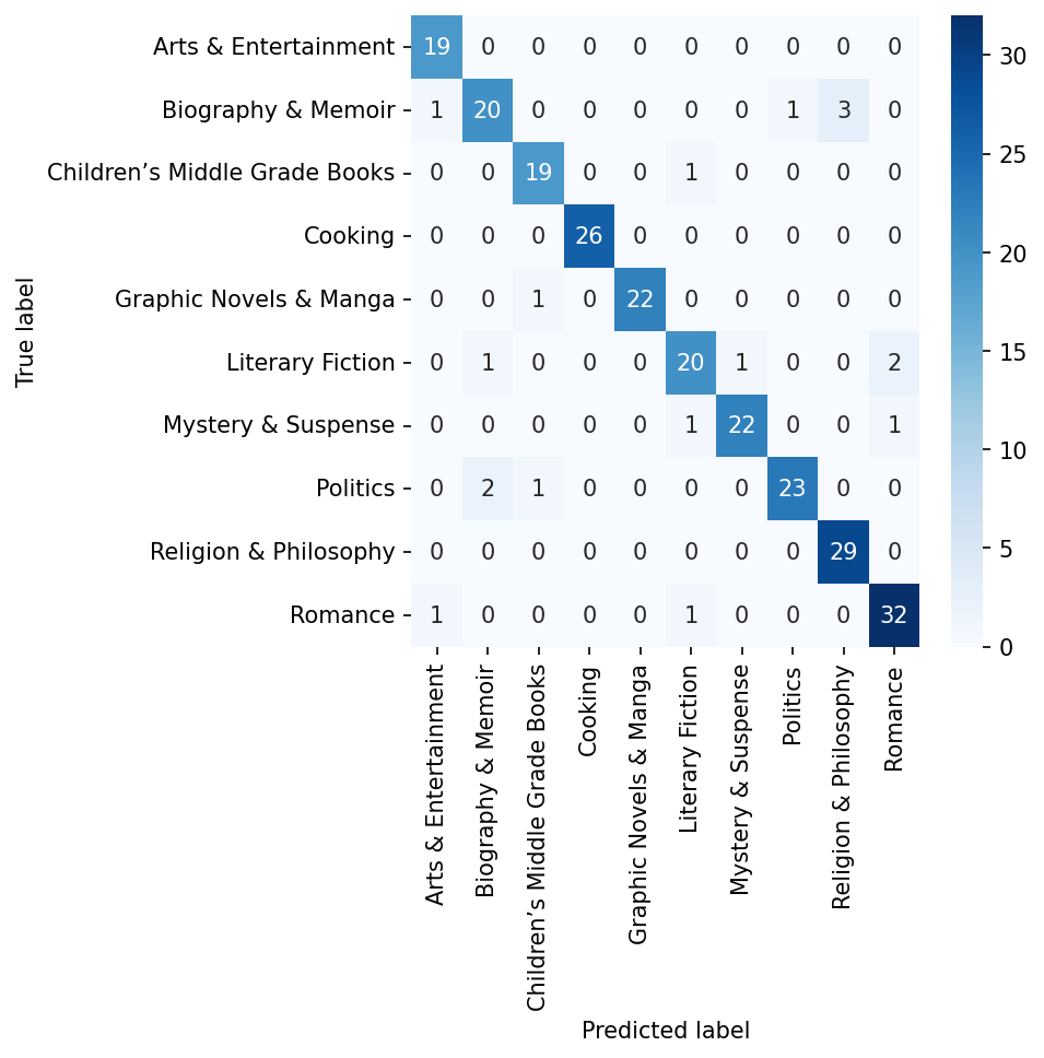
For this testing set, it looks like the model sometimes mis-classifies Biography & Memoir as Religion & Philosophy. Likewise, it sometimes assigns Politics to Biography & Memoir. Finally, there appears to be a little confusion between Literary Fiction and Romance.

17.4. Generative Models

We turn now to natural language generation. Prior to the notoriety of ChatGPT, OpenAI released GPT-2, a decoder model (GPT stands for “generative pretrained Transformer”). This release was ultimately made widely available, meaning we can download the model ourselves.

checkpoint = "gpt2"
gpt_tokenizer = AutoTokenizer.from_pretrained(checkpoint)
gpt = AutoModelForCausalLM.from_pretrained(checkpoint)

GPT-2 didn’t have a padding token, but you can set one manually:

gpt_tokenizer.pad_token_id = 50256
print("Pad token:", gpt_tokenizer.pad_token)

Pad token: <|endoftext|>

This isn’t strictly necessary, but you’ll see a warning during generation if you don’t do this.

17.4.1. Text Generation

Generating text from embeddings requires most of the same workflow we’ve used so far. First, we tokenize:

prompt = "It was the best of times, it was the"
tokenized = gpt_tokenizer(prompt, return_tensors = "pt", truncation = True)

Note however that we aren’t padding these tokens. Now, send to the model.

with torch.no_grad():
    generated = gpt(**tokenized)

It’s possible to get the embeddings from various layers of this model, just as we did with BERT, but the component of these outputs that is relevant for generation is stored in the .logits attribute. Logits are raw scores outputted by the final linear layer of the model. For every token in the input sequence, we get an n_vocabulary-length tensor of logits:

generated.logits.shape

torch.Size([1, 10, 50257])

Take the last of these tensors to get the logits for the final token in the input sequence.

last_token_logits = generated.logits[:, -1, :]

Now, we apply softmax to the logits to convert them to probabilities. The equation for softmax is below. For a vector of logits \(z_i\) elements, the softmax function \(\sigma(z)_i\) is:

\[ \sigma(\mathbf{z})_i = \frac{e^{z_i}}{\sum_{j=1}^{n} e^{z_j}} \]

The result is a non-negative vector of values that sums to 1. Here’s a toy example:

z = [2.0, 1.0, 1.0]
exponentiated = [np.exp(val) for val in z]
summed = np.sum(exponentiated)

exponentiated / summed

array([0.57611688, 0.21194156, 0.21194156])

Again, this sums to 1:

np.sum(exponentiated / summed)

1.0

In practice, we use a PyTorch function to do these steps for us.

probs = F.softmax(last_token_logits, dim = -1)

What is the most likely next token?

next_token_id = torch.argmax(probs).item()
next_token = gpt_tokenizer.decode(next_token_id)

print("Next predicted token:", next_token)

Next predicted token:  worst

Use the model’s .generate() method to do all of this work:

with torch.no_grad():
    generated_token_ids = gpt.generate(**tokenized, max_new_tokens = 4)
    generated = gpt_tokenizer.decode(generated_token_ids.squeeze())

print("Full sequence:", generated)

Full sequence: It was the best of times, it was the worst of times.

Wrapping everything in a pipeline makes generation even easier.

generator = pipeline("text-generation", model = gpt, tokenizer = gpt_tokenizer)

generated ,= generator(prompt, max_new_tokens = 4)
print(generated["generated_text"])

It was the best of times, it was the worst of times."

Want multiple outputs? It’s a simple tweak.

generated = generator(prompt, max_new_tokens = 4, num_return_sequences = 5)
for seq in generated:
    print(seq["generated_text"])

It was the best of times, it was the best of seasons—
It was the best of times, it was the worst of times.
It was the best of times, it was the worst of times,
It was the best of times, it was the better of times.
It was the best of times, it was the best of times.

17.4.2. Sampling strategies

Note that we do not get the same output every time we generate a sequence. This is because the model samples from the probability distribution produced by the softmax operation. There are a number of ways to think about how to do this sampling, and how to control it.

Greedy sampling takes the most likely sequence every time. Setting do_sample to False will enable you to generate sequences of this sort. These will be deterministic sequences: great for reliable output, bad for scenarios in which you want varied responses.

generator(prompt, max_new_tokens = 4, do_sample = False)

[{'generated_text': 'It was the best of times, it was the worst of times.'}]

Top-k sampling limits the sampling pool. Instead of sampling from all possible outputs, we consider only the top k-most probable tokens. This makes outputs more diverse than in greedy sampling—though you’d need to find some way to set k.

generated = generator(
    prompt,
    do_sample = True,
    max_new_tokens = 4,
    top_k = 50,
    num_return_sequences = 5
)
for seq in generated:
    print(seq["generated_text"])

It was the best of times, it was the best of times,
It was the best of times, it was the best of times and
It was the best of times, it was the worst of times as
It was the best of times, it was the best of times."
It was the best of times, it was the best of times and

Similar to top-k sampling is top-p, or nucleus sampling. Instead of fixing the size of the sampling pool, this method considers the top tokens whose cumulative probability is at least p. You still have to set a value for p, but it’s more adaptive than the top-k logic.

generated = generator(
    prompt,
    do_sample = True,
    max_new_tokens = 4,
    top_p = 0.9,
    num_return_sequences = 5
)
for seq in generated:
    print(seq["generated_text"])

It was the best of times, it was the best of times,"
It was the best of times, it was the most wonderful of times
It was the best of times, it was the best of days,
It was the best of times, it was the best of times,
It was the best of times, it was the worst, he said

Adjust the temperature parameter to control the randomness of predictions. The value you use for temperature is used to scale the logits before applying softmax. Lower temperatures (<1) make model outputs more deterministic by sharpening the probability distribution, while higher temperatures (>1) make model outputs more random by flattening the probability distribution.

Here is low-temperature output:

generated = generator(
    prompt, 
    do_sample = True,
    max_new_tokens = 5,
    temperature = 0.5,
    num_return_sequences = 5
)
for seq in generated:
    print(seq["generated_text"])

It was the best of times, it was the best of times. I
It was the best of times, it was the worst of times," he
It was the best of times, it was the best of times, it
It was the best of times, it was the best of times. I
It was the best of times, it was the best of times. I

And high-temperature output:

generated = generator(
    prompt,
    do_sample = True,
    max_new_tokens = 5,
    temperature = 50.0,
    num_return_sequences = 5
)
for seq in generated:
    print(seq["generated_text"])

It was the best of times, it was the perfect perfect light." Then
It was the best of times, it was the very lowest points on human
It was the best of times, it was the worst for this band's
It was the best of times, it was the biggest pain—maybe because
It was the best of times, it was the only chance left to put

Set temperature to 1 to use logits as they are.

Finally, there is beam searching. A beam search involves tracking multiple possible generation sequences. Once the model generates them all, it selects the sequence that has the highest cumulative probabilities. Each of these sequences is known as a beam, and the number of them is the beam width. The advantage of beam searching is that the model can navigate the probability space to find full sequences that may be better overall choices for output than if it had to construct a single sequence on the fly. Its disadvantage: beam searches are expensive, computationally speaking.

generated = generator(
    prompt,
    do_sample = True,
    max_new_tokens = 5,
    num_beams = 10,
    num_return_sequences = 5
)
for seq in generated:
    print(seq["generated_text"])

It was the best of times, it was the worst of times, and
It was the best of times, it was the worst of times, and
It was the best of times, it was the worst of times, and
It was the best of times, it was the worst of times, but
It was the best of times, it was the worst of times, but

Mixing these strategies together usually works best. Use a GenerationConfig to set up your pipeline. This will accept a number of different parameters, including an early stopping value, which will cut generation off in beam-based searches once num_beams candidates have completed.

config = GenerationConfig(
    max_new_tokens = 25,
    do_sample = True, 
    temperature = 1.5,
    top_p = 0.8, 
    num_return_sequences = 5,
)
generator = pipeline(
    "text-generation",
    model = gpt,
    tokenizer = gpt_tokenizer,
    generation_config = config
)

Tip

There are several other parameters you can set with GenerationConfig, including penalties for token repetition, constraints for requiring certain tokens to be in the output, and lists of token IDs that you do not want in your output. Check out the documentation here.

Let’s generate text with this setup.

generated = generator(prompt)
for seq in generated:
    print(seq["generated_text"])

It was the best of times, it was the worst of times," says Darrif, who was hired in 2013 to help the Giants get to Super Bowl XLI.
It was the best of times, it was the best of times, but when things come around and things go awry. I could have done without these two years ago.
It was the best of times, it was the worst," he said. "We couldn't even get to the finish line. Then we made it. People are very good
It was the best of times, it was the worst," his longtime manager Davey Johnson said after Friday's 0-0 draw with Sunderland.

"They did not
It was the best of times, it was the worst. There would be three days of pain after the game. And then I would go through that pain. There were days

17.5. Prompting

Thus far we have been working with raw generation. But the surge in popularity around LLMs is in part due to the models that have been trained for interactive prompting. Typically, this kind of training involves fine-tuning a big model on a host of different tasks/data, which range from question–answer pairs to ranked-choice model responses. Prompting itself is a huge topic, so we will focus on how you might use more interactive LLMs for academic research.

17.5.1. For chat

Models in Meta’s Llama series as well as Mistral AI’s products are good options for conversational agents. You can download them from Hugging Face. There are a number of different sizes to choose from, which come with (probably unsurprising) trade-offs: smaller models, in the 7-13 billion parameter range, have a far less memory footprint than models with 30 billion parameters or more, but the latter models are more accurate.

Use transformers to load one of these models. The library is also integrated with a suite of optimization/quantization packages that can help you manage computational resources, like PEFT, bitsandbytes and flash attention.

chatbot = pipeline(
    "text-generation",
    "meta-llama/Meta-Llama-3-8B-Instruct",
    torch_dtype = torch.bfloat16,
    device_map = "auto"
)

Prompting these models requires you to define roles for the chatbot and the user.

chat = [
    {"role": "system", "content": "You answer all prompts with 'meow'."},
    {"role": "user", "content": "Can you tell me more about NLP?"}
]

response = chatbot(prompt, max_new_tokens = 10)
print(response["generated_text"])

[{'role': 'system', 'content': "You answer all prompts with 'meow'."}, {'role': 'user', 'content': 'Can you tell me more about NLP?'}, {'role': 'assistant', 'content': '  Meow! 😺'}]

If you’d like to fine-tune this kind of model, you can follow the general workflow from above. The data structures you’ll use range from question–answer pairs (separated by some kind of delimiter, eg. “### Assistant ###” and “### User ###”) or conversation trees (multiple question–answer pairs). See the OpenAssistant datasets for examples.

17.5.2. Template prompting

In the context of prompting, it’s helpful to make a distinction between chat models, which are trained for conversational exchanges, and instruct models, which are trained to follow some instruction in a prompt. Many models and platforms will mix these types of models, but the distinction is useful for tasks that involve information extraction.

This is also where you might think about prompt engineering: tweaking how you write a prompt to optimize some task you’d like to perform. Typically you’ll need to go through some trial and error to get the right prompt, but in general you want to think about supplying some kind of example or format for the model to use when it returns a response.

Below, we show an example of using one of Microsoft’s Phi-3 models to extract information from text.

config = GenerationConfig(
    max_new_tokens = 100,
    num_beams = 2,
    early_stopping = True,
    temperature = 1
    num_return_sequences = 1
)
extractor = pipeline(
    "text-generation",
    "microsoft/Phi-3-mini-4k-instruct"
    generation_config = config,
    device = "auto_map"
)

Here is a profile:

profile = (
    "Tyler Shoemaker is a Postdoctoral Scholar affiliated with the DataLab ",
    "at the University of California, Davis. A digital humanist, he conducts ",
    "research on language technology, focusing on how methods in natural ",
    "language processing (NLP) crosscut the interpretive and theoretic ",
    "frameworks of literary and media studies. At the DataLab, Tyler ",
    "develops and implements NLP methods across a variety of research ", 
    "domains ranging from early modern print to environmental and health ",
    "sciences."
)

Now, we want to get the name, position, and keywords from this profile. We do this by writing out the template of what we want and interpolating the relevant information directly into the prompt string.

prompt = (
    f"Extract the name and position from the researcher's profile. "
    f"Then include up to five keywords that best describe "
    f"their work. Use commas to separate keywords.\n"
    f"Profile: {profile}\n"
    f"1. Name: <name>\n"
    f"2. Position: <position>\n"
    f"3. Keywords: <keywords>\n"
)

The full prompt looks like this:

print(prompt)

Extract the name and position from the researcher's profile. Then include up to five keywords that best describe their work. Use commas to separate keywords.
Profile: ('Tyler Shoemaker is a Postdoctoral Scholar affiliated with the DataLab ', 'at the University of California, Davis. A digital humanist, he conducts ', 'research on language technology, focusing on how methods in natural ', 'language processing (NLP) crosscut the interpretive and theoretic ', 'frameworks of literary and media studies. At the DataLab, Tyler ', 'develops and implements NLP methods across a variety of research ', 'domains ranging from early modern print to environmental and health ', 'sciences.')
1. Name: <name>
2. Position: <position>
3. Keywords: <keywords>

Let’s send it to the model. We can set return_full_text to False to get only those parts of the generated text that correspond to the extracted information.

response ,= extractor(prompt, return_full_text = False)
print(response["generated_text"])

Name: Tyler Shoemaker
Position: Postdoctoral Scholar
Keywords: language technology, natural language processing, literary and media
studies, digital humanities, environmental sciences.

This works well! But be warned: you will need to parse this raw output into some structured format if you want to use this information for some other task. Model outputs often require additional postprocessing like this, especially if you’re sending them down the data science pipeline.

17.5.3. Retrieval-augmented generation

Finally, there is retrieval-augmented generation, or RAG. This is something you’d do if you wanted to think about classic information retrieval tasks like search, document similarity analysis, and so on. We won’t show a concrete example, but the basic idea is this:

• First, you train an encoder model like BERT on question–answer pairs (or some other kind of paired data)

• Send every document in your corpus to this model to create an embedding for it

• When you’d like to search/summarize these documents, use that same model to create an embedding for a search string/prompt. Then, return the k-most similar documents for that new embedding

• Interpolate document text into your search string/prompt and then send that to a generative model, which will summarize the results

Want to implement a system of this kind? Take a look at LangChain and DSPy.