3. Cleaning and Counting#
At the end of the last chapter, we briefly discussed the complexities involved in working with textual data. Textual data presents a number of challenges – which stem as much from general truths about language as they do from data representations – that we need to address so that we can formalize text in a computationally tractable manner.
This formalization enables us to count words. Nearly all methods in text analytics begin by counting the number of times a word occurs and by taking note of the context in which that word occurs. With these two pieces of information, counts and context, we can identify relationships among words and, on this basis, formulate interpretations.
This chapter will discuss how to wrangle the messiness of text so we can count it. We’ll continue with Frankenstein and learn how to prepare text so as to generate valuable metrics about the words within the novel (later sessions will use these metrics for multiple texts).
Learning Objectives
By the end of this chapter, you will be able to:
Clean textual data
Recognize how cleaning changes the findings of text analysis
Implement preliminary counting operations on cleaned text
Use a statistical measure (pointwise mutual information) to measure unique phrases
3.1. Preliminaries#
3.1.1. Overview#
Think back to the end of the last chapter. There, we discussed differences between how computers represent and process text and our own way of reading. A key difference involves details like spelling and capitalization. For us, the meaning of text tends to cut across these details. But they make all the difference in how computers track information. So, if we want to work at a higher order of meaning, not just character sequences, we need to eliminate as many variances as possible in textual data.
Eliminating these variances is known as cleaning text. The entire process typically happens in steps, which include:
Resolving word cases
Removing punctuation
Removing numbers
Removing extra whitespaces
Removing stop words
Note though that there is no pre-set way to clean text. The steps you need to perform all depend on your data and the questions you have. We’ll walk through each of these steps below and, along the way, compare how they alter the original text to show why you might (or might not) implement them.
3.1.2. Setup#
To make these comparisons, load in Frankenstein.
with open("data/session_one/shelley_frankenstein.txt", 'r') as fin:
    frankenstein = fin.read()
And import some libraries.
import re
from collections import Counter
import nltk
from nltk.stem.porter import PorterStemmer
from nltk.stem.wordnet import WordNetLemmatizer
from nltk import collocations
import pandas as pd
import matplotlib.pyplot as plt
import seaborn as sns
Finally, define a simple function to count words. This will help us quickly check the results of a cleaning step.
def count_words(doc):
    """Count words in a document."""
    doc = doc.split()
    counts = Counter(doc)

    return counts
Let’s use this function to get the original number of words in Frankenstein.
counts = count_words(frankenstein)
print("Unique words:", len(counts))
Unique words: 11590
3.2. Basic Cleaning#
3.2.1. Case normalization#
The first step in cleaning is straightforward. Since computers are case-sensitive, we need to convert all characters to upper- or lowercase. It’s standard to change all letters to their lowercase forms.
uncased = frankenstein.lower()
This should reduce the number of unique words.
uncased_counts = count_words(uncased)
print("Unique words:", len(uncased_counts))
Unique words: 11219
Double check: will we face the same problems from the last chapter?
print("'Letter' in `uncased`:", ("Letter" in uncased_counts))
print("Number of times 'the' appears:", uncased_counts['the'])
'Letter' in `uncased`: False
Number of times 'the' appears: 4152
So far so good. Now, “the” has become even more prominent in the counts: there are ~250 more instances of this word after changing its case (it was 3,897 earlier).
3.2.2. Removing Punctuation#
Time to tackle punctuation. This step is trickier and it typically involves some back and forth between inspecting the original text and the output. This is because punctuation marks have different uses, so they can’t all be handled the same way.
Consider the following:
s = "I'm a self-taught programmer."
It seems most sensible to remove punctuation with some combination of regular
expressions, or “regex,” with re.sub(), which substitutes a regex
sequence with something else. For example, using regex to remove anything that
is not (^) a word (\w) or a space (\s) will give the following:
print(re.sub(r"[^\w\s]", "", s))
Im a selftaught programmer
This method has its advantages. It sticks the m in “I’m” back to the I. While this isn’t perfect, as long as we remember that, whenever we see “Im,” we mean “I’m,” it’s doable. That said, this method also sticks “self” and “taught” together, which we don’t want. It would be better to separate those two words than create a new one altogether. Ultimately, this is a tokenization question: what do we define as acceptable tokens in our data, and how are we going to create those tokens?
Different NLP libraries in Python will handle this question in different ways.
For example, the word_tokenize() function from nltk returns the following:
nltk.word_tokenize(s)
['I', "'m", 'a', 'self-taught', 'programmer', '.']
See how it handles punctuation differently, depending on the string?
In our case, we’ll want to separate phrases like “self-taught” into their components. The best way to do so is to process punctuation marks in stages. First, remove hyphens, then remove other punctuation marks.
s = re.sub(r"-", " ", s)
s = re.sub(r"[^\w\s]", "", s)
print(s)
Im a self taught programmer
Let’s use the same logic on Frankenstein. Note that we’re actually removing two different kinds of hyphens, the en dash (-) and the em dash (—). We also use different replacement strategies depending on the type of character.
no_punct = re.sub(r"[-—]", " ", uncased)
no_punct = re.sub(r"[^\w\s]", "", no_punct)
Finally, we remove underscores, which regex classes as word characters. The
expression ^\w does not capture this punctuation.
no_punct = re.sub(r"_", "", no_punct)
Tip
If you didn’t want to do this separately, you could always include underscores in your code for handling hyphens. That said, punctuation removal is almost always a multi-step process, the honing of which involves multiple iterations.
With punctuation removed, here is the text:
print(no_punct[:351])
letter 1

to mrs saville england


st petersburgh dec 11th 17


you will rejoice to hear that no disaster has accompanied the
commencement of an enterprise which you have regarded with such evil
forebodings i arrived here yesterday and my first task is to assure
my dear sister of my welfare and increasing confidence in the success
of my undertaking
3.2.3. Removing numbers#
Removing numbers presents less of a problem. All we need to do is find characters 0-9 and replace them.
no_punctnum = re.sub(r"[0-9]", "", no_punct)
Now that we’ve removed punctuation and numbers, unique word counts should significantly decrease. This is because we’ve separated these characters from word sequences, so “letter:” and “letter.” will count as “letter.”
no_punctnum_counts = count_words(no_punctnum)
print("Unique words:", len(no_punctnum_counts))
Unique words: 6992
That’s nearly a 40% reduction in the number of unique words!
3.2.4. Text formatting#
Our punctuation and number removal introduced extra whitespaces in the text
(recall that we used a whitespace as a replacement character for some
punctuation). We need to remove those, along with newlines and tabs. There are
regex patterns for doing so, but Python’s .split() method captures all
whitespace characters. In fact, the count_words() function above has been
doing this all along. So tokenizing our text as before will also take care of
this step.
cleaned = no_punctnum.split()
With that, we are back to the list representation of Frankenstein that we worked with in the last chapter – but this time, our metrics are much more robust. Here are the top 25 words:
cleaned_counts = Counter(cleaned)
for entry in cleaned_counts.most_common(25):
    print(entry)
('the', 4194)
('and', 2976)
('i', 2850)
('of', 2642)
('to', 2094)
('my', 1776)
('a', 1391)
('in', 1129)
('was', 1021)
('that', 1017)
('me', 867)
('but', 687)
('had', 686)
('with', 667)
('he', 608)
('you', 574)
('which', 558)
('it', 547)
('his', 535)
('as', 528)
('not', 510)
('for', 498)
('by', 460)
('on', 460)
('this', 402)
3.3. Stopword Removal#
With the first few steps of our cleaning done, let’s pause and look more closely at our output. Inspecting the counts above shows a pattern: nearly all of them are deictic words, or words that are highly dependent on the context in which they appear. We use these words constantly to refer to specific times, places, and persons – indeed, they’re the very sinew of language, and their high frequency counts reflect this.
3.3.1. High frequency words#
Plotting word counts shows the full extent of these high frequency words. Below, we define a function to show them.
def plot_counts(counts, n_words = 200, by_x = 10):
    """Plot word counts."""
    counts = pd.DataFrame(counts.items(), columns = ('word', 'count'))
    counts.sort_values('count', ascending = False, inplace = True)

    fig, ax = plt.subplots(figsize = (9, 6))
    g = sns.lineplot(x = 'word', y = 'count', data = counts[:n_words], ax = ax)
    g.set(xlabel = "Words", ylabel = "Counts")
    plt.xticks(rotation = 90, ticks = range(0, n_words, by_x));

plot_counts(cleaned_counts, len(cleaned_counts), 150)
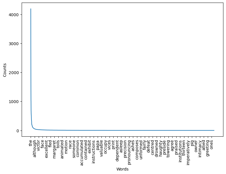
See that giant drop? Let’s look at the 200-most frequent words.
plot_counts(cleaned_counts, 200, 5)
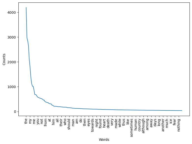
Only a few non-deictic words appear in the first half of this graph – “eyes,” “night,” “death,” for example. All others are words like “my,” “from,” etc. And this second set of words have incredibly high frequency counts. In fact, the 50-most frequent words in Frankenstein comprise nearly 50% of the total number of words in the novel!
top50 = sum(count for word, count in cleaned_counts.most_common(50))
total = cleaned_counts.total()
print(f"Percentage of 50-most frequent words: {top50 / total * 100:.02f}%")
Percentage of 50-most frequent words: 47.71%
The problem here is that, even though these high frequency words help us mean what we say, they paradoxically don’t seem to have much meaning in and of themselves. These words are so common and so context-dependent that it’s difficult to find much to say about them in isolation. Worse still, every novel we put through the above analyses is going to have a very similar distribution in terms – they’re just a general fact of language.
We need a way to handle these words. The most common way to do this is to remove them altogether. This is called stopping the text. But how do we know which stopwords to remove?
3.3.2. Defining a stop list#
The answer comes in two parts. First, compiling various stop lists has been an ongoing research area in NLP since the emergence of information retrieval in the 1950s. There are several popular lists, which capture many of the words we’d think to remove: “the,” “do,” “as,” etc. Popular NLP packages even come preloaded with generalized lists; we’ll be using one compiled by the developers of Voyant, a text analysis portal.
with open("data/voyant_stoplist.txt", 'r') as fin:
    stopwords = fin.read().split("\n")

print(stopwords[:10])
['a', 'about', 'above', 'across', 'after', 'afterwards', 'again', 'against', 'all', 'almost']
Removing stopwords can be done with a list comprehension:
stopped = [word for word in cleaned if word not in stopwords]
stopped_counts = Counter(stopped)
plot_counts(stopped_counts, 200, 5)
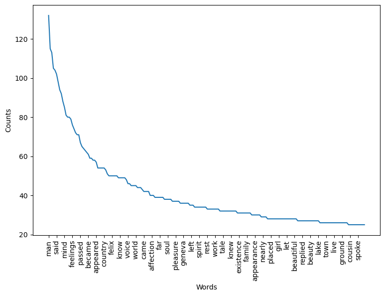
This is looking good, but it would be nice if we could also remove “said” from our text. Doing so brings us to the second, and most important part of the answer to the question, which stopwords should we use? In truth, removing stopwords depends on your texts and your research question(s). We’re looking at a novel, so we know there will be a lot of dialogue. But dialogue markers aren’t useful for understanding something a concept like topicality (i.e. what the novel is about). So, we’ll remove those markers.
But in other texts, or with other research questions, we might not want to do so. A good stop list, then, is application-specific. You may in fact find yourself using different stop lists for different parts of a project.
That all said, there are a broad set of NLP tasks that can really depend on keeping stopwords in your text. These are tasks that fall under part-of-speech tagging: they rely on stopwords to parse the grammatical structure of text. Below, we will discuss one such example of these tasks, though for now, we’ll go ahead with our current stop list.
Let’s add “said” to our stop list, redo the stopping process, and count the results. Note that it’s also customary to remove words that are two characters long or less (this prevents us from seeing things like “st,” for street).
stopwords += ['said']
stopped = [word for word in cleaned if word not in stopwords]
stopped = [word for word in stopped if len(word) > 2]
stopped_counts = Counter(stopped)
plot_counts(stopped_counts, 200, 5)
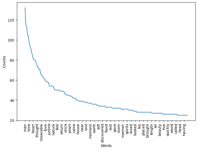
Finally, here are the 50-most frequent words from our completely cleaned text:
for entry in stopped_counts.most_common(50):
    print(entry)
('man', 132)
('life', 115)
('father', 113)
('shall', 105)
('eyes', 104)
('time', 98)
('saw', 94)
('night', 92)
('elizabeth', 88)
('mind', 85)
('heart', 81)
('day', 80)
('felt', 80)
('death', 79)
('feelings', 76)
('thought', 74)
('dear', 72)
('soon', 71)
('friend', 71)
('passed', 67)
('miserable', 65)
('place', 64)
('like', 63)
('heard', 62)
('became', 61)
('love', 59)
('clerval', 59)
('little', 58)
('human', 58)
('appeared', 57)
('country', 54)
('misery', 54)
('words', 54)
('friends', 54)
('justine', 54)
('nature', 53)
('cottage', 51)
('feel', 50)
('great', 50)
('old', 50)
('away', 50)
('hope', 50)
('felix', 50)
('return', 49)
('happiness', 49)
('know', 49)
('days', 49)
('despair', 49)
('long', 48)
('voice', 46)
3.4. Advanced Cleaning#
With stopwords removed, all primary text cleaning steps are complete. But there are two more steps that we could perform to further process our data: stemming and lemmatizing. We’ll consider these separately from the steps above because they entail making significant changes to our data. Instead of simply removing pieces of irrelevant information, as with stopword removal, stemming and lemmatizing transform the forms of words.
3.4.1. Stemming#
Stemming algorithms are rule-based procedures that reduce words to their root forms. They cut down on the amount of morphological variance in a corpus, merging plurals into singulars, changing gerunds into static verbs, etc. As with the steps above, stemming a corpus cuts down on lexical variety. More, it enacts a shift to a generalized form of words’ meanings: instead of counting “have” and “having” as two different words with two different meanings, stemming would enable us to count them as a single entity, “have.”
nltk implements stemming with its PorterStemmer. It’s a class object, which
must be initialized by saving it to a variable.
stemmer = PorterStemmer()
Let’s look at a few words.
to_stem = ('books', 'having', 'running', 'complicated', 'complicity')
for word in to_stem:
    print(f"{word:<12} => {stemmer.stem(word)}")
books        => book
having       => have
running      => run
complicated  => complic
complicity   => complic
There’s a lot of potential value in enacting these transformations. So far we haven’t developed a method for handling plurals; the stemmer can take care of them. Likewise, it usefully merges “have” with “having.” It would be difficult to come up with a custom algorithm that could handle the complexities of such a transformation.
That said, the problem with stemming is that the process is rule-based and struggles with certain words. It can inadvertently merge what should be two separate words, as with “complicated” and “complicity” both becoming “complic.” And more, “complic” isn’t really a word. How would we know what it means when looking at word distributions?
3.4.2. Lemmatizing#
Lemmatizing solves some of these problems, though at the cost of more complexity. Like stemming, lemmatization removes the inflectional forms of words. While it tends to be more conservative in its approach, it is better at avoiding lexical merges like “complic.” More, the result of lemmatization is always a fully readable word.
3.4.2.2. Sample lemmatization workflow#
We won’t do all of this for Frankenstein, but in the next session, when we
start to use classification models to understand the difference between texts,
we’ll do so using texts cleaned according to the above workflow. For now, we’ll
demonstrate an example of POS tagging using the nltk tokenizer in concert
with its lemmatizer.
example = """The strong coffee, which I had after lunch, was $3.
It kept me going the rest of the day."""

tokenized = nltk.word_tokenize(example)
for token in tokenized:
    print(token)
The
strong
coffee
,
which
I
had
after
lunch
,
was
$
3
.
It
kept
me
going
the
rest
of
the
day
.
Assigning POS tags:
tagged = nltk.pos_tag(tokenized)
for token in tagged:
    print(token)
('The', 'DT')
('strong', 'JJ')
('coffee', 'NN')
(',', ',')
('which', 'WDT')
('I', 'PRP')
('had', 'VBD')
('after', 'IN')
('lunch', 'NN')
(',', ',')
('was', 'VBD')
('$', '$')
('3', 'CD')
('.', '.')
('It', 'PRP')
('kept', 'VBD')
('me', 'PRP')
('going', 'VBG')
('the', 'DT')
('rest', 'NN')
('of', 'IN')
('the', 'DT')
('day', 'NN')
('.', '.')
Time to lemmatize. We do so in two steps. First, we need to convert the POS
tags nltk produces to tags that this lemmatizer expects. We did say this is
more complicated!
wordnet = nltk.corpus.wordnet

def convert_tag(tag):
    """Convert a TreeBank tag to a WordNet tag."""
    if tag.startswith('J'):
        tag = wordnet.ADJ
    elif tag.startswith('V'):
        tag = wordnet.VERB
    elif tag.startswith('N'):
        tag = wordnet.NOUN
    elif tag.startswith('R'):
        tag = wordnet.ADV
    else:
        tag = ''

    return tag

tagged = [(word, convert_tag(tag)) for (word, tag) in tagged]
Now we can lemmatize.
lemmatizer = WordNetLemmatizer()

def lemmatize(word, tag):
    """Lemmatize a word."""
    if tag:
        return lemmatizer.lemmatize(word, pos = tag)

    return lemmatizer.lemmatize(word)

lemmatized = [lemmatize(word, tag) for (word, tag) in tagged]
Joining the list entries back into a string will give the following:
joined = " ".join(lemmatized)
print(joined)
The strong coffee , which I have after lunch , be $ 3 . It keep me go the rest of the day .
From here, pass this string back through the cleaning steps we’ve already covered.
3.5. Chunking with N-Grams#
We are now finished cleaning text. The last thing we’ll discuss in this session is chunking. Chunking is closely related to tokenization. It involves breaking text into multi-token spans. This is useful if you want to find phrases in data, or even entities. For example, all the steps above would dissolve “New York” into “new” and “york.” A multi-token span, on the other hand, would keep this string intact.
In this sense, it’s often useful to count not only single words in text, but continuous two-word strings, or even longer ones. These strings are called n-grams, where n is the number of tokens in the span. “Bigrams” are two-token spans. “Trigrams” have three tokens, while “4-grams” and “5-grams” have four and five tokens, respectively. Technically, there’s no limit to n-gram sizes, though their usefulness depend on your data and research questions.
To finish this chapter, we’ll produce bigram counts on Frankenstein. nltk
has built-in functionality to help us do so. There are a few options here.
We’ll use objects from the collocations module.
A BigramCollocationFinder will find the bigrams.
finder = collocations.BigramCollocationFinder.from_words(stopped)
Access its ngram_fd attribute for counts, which we’ll store in a pandas
DataFrame.
bigrams = finder.ngram_fd

bigrams = [(word, pair, count) for (word, pair), count in bigrams.items()]
bigrams = pd.DataFrame(bigrams, columns = ('word', 'pair', 'count'))
bigrams.sort_values('count', ascending = False, inplace = True)
Top bigrams:
bigrams.head(10)
| word | pair | count | |
|---|---|---|---|
| 826 | old | man | 32 |
| 623 | native | country | 15 |
| 3333 | natural | philosophy | 14 |
| 6999 | taken | place | 13 |
| 5901 | fellow | creatures | 12 |
| 3395 | dear | victor | 10 |
| 6784 | short | time | 9 |
| 7606 | young | man | 9 |
| 2631 | long | time | 9 |
| 2434 | poor | girl | 8 |
Looks good! Some phrases are peeking through. But while raw counts provide us with information about frequently occurring phrases in text, it’s hard to know how unique these phrases are. For example, “man” appears throughout the novel, so it’s likely to appear in many bigrams. How, then, might we determine whether there’s something unique about whether “old” and “man” consistently stick together?
One way to do this is with a PMI, or pointwise mutual information, score. PMI measures the association strength of a pair of outcomes. In our case, the higher the score, the more likely a given bigram pair will be with respect to the other bigrams in which the two words of the one under consideration.
We can get a PMI score for each bigram using our finder’s .score_ngrams()
method in concert with a BigramAssocMeasures object; we send the latter as an
argument to the former. As before, let’s format the result for a pandas
DataFrame.
measures = collocations.BigramAssocMeasures()

bigram_pmi = finder.score_ngrams(measures.pmi)
bigram_pmi = [(word, pair, val) for (word, pair), val in bigram_pmi]
bigram_pmi = pd.DataFrame(bigram_pmi, columns = ('word', 'pair', 'pmi'))
bigram_pmi.sort_values('pmi', ascending = False, inplace = True)
10 bottom-most scoring bigrams:
bigram_pmi.tail(10)
| word | pair | pmi | |
|---|---|---|---|
| 29025 | eyes | eyes | 1.491758 |
| 29026 | eyes | shall | 1.477952 |
| 29027 | man | saw | 1.293655 |
| 29028 | saw | man | 1.293655 |
| 29029 | father | father | 1.252280 |
| 29030 | life | father | 1.226969 |
| 29031 | man | eyes | 1.147804 |
| 29032 | man | shall | 1.133998 |
| 29033 | shall | man | 1.133998 |
| 29034 | man | father | 1.028065 |
And 10 random bigrams with scores above the 75th percentile.
bigram_pmi[bigram_pmi['pmi'] > bigram_pmi['pmi'].quantile(0.75)].sample(10)
| word | pair | pmi | |
|---|---|---|---|
| 4519 | sense | term | 11.307675 |
| 6457 | sufficient | conquer | 10.570710 |
| 5677 | boy | singular | 10.722713 |
| 3775 | perilous | situation | 11.570710 |
| 429 | aspired | omnipotence | 13.892638 |
| 4198 | dome | mont | 11.307675 |
| 5751 | expiration | month | 10.722713 |
| 4517 | sensation | helplessness | 11.307675 |
| 3360 | enters | cabin | 11.722713 |
| 473 | colonization | trade | 13.892638 |
Among the worst-scoring bigrams there are words that are likely to appear alongside many different words: “said,” “man,” “shall,” etc. On the other hand, among the best-scoring bigrams there are coherent entities and suggestive pairings. The latter especially begin to sketch out the specific qualities of Shelley’s prose style.