6. Topic Modeling

This final chapter follows from the previous chapter’s use of cosine similarity. The latter used this metric to cluster obituaries into broad categories based on what those obituaries were about. Similarly, in this chapter we’ll use topic modeling to identify the thematic content of a corpus and, on this basis, associate themes with individual documents.

As we’ll discuss below, human interpretation plays a key role in this process: topic models produce textual structures, but it’s on us to give those structures meaning. Doing so is an iterative process, in which we fine tune various aspects of a model to effectively represent our corpus. This chapter will show you how to build a model, how to appraise it, and how to start iterating through the process of fine tuning to produce a model that best serves your research questions.

To do so, we’ll use a corpus of book blurbs sampled from the U. Hamburg Language Technology Group’s Blurb Genre Collection. The collection contains ~92,000 blurbs from Penguin Random House, ranging from Colson Whitehead’s books to steamy supermarket romances and self-help manuals. We’ll use just 1,500 – not so much that we’d be stuck waiting for hours for models to train, but enough to get a broad sense of different topics among the blurbs.

Learning Objectives

By the end of this chapter, you will be able to:

• Explain what a topic model is, what it represents, and how to use one to explore a corpus

• Build a topic model

• Use two scoring metrics, perplexity and coherence, to appraise the quality of a model

• Understand how to improve a model by fine tuning its number of topics and its hyperparameters

6.1. How It Works

Citations

This description of topic modeling is influenced by Ted Underwood’s very effective explanation. This review article, from David M. Blei (one of the original developers of the method), is also quite helpful.

There are a few different flavors of topic models. We’ll be using the most popular one, a latent Dirichlet allocation, or LDA, model. It involves two assumptions: 1) documents are comprised of a mixture of topics; 2) topics are comprised of a mixture of words. An LDA model represents these mixtures in terms of probability distributions: a given passage, with a given set of words, is more or less likely to be about a particular topic, which is in turn more or less likely to be made up of a certain grouping of words.

We initialize a model by predefining how many topics we think it should find. When the model begins training, it randomly guesses which words are most associated with which topic. But over the course of its training, it will start to keep track of the probabilities of recurrent word collocations: “river”, “bank,” and “water,” for example, might keep showing up together. This suggests some coherence, a possible grouping of words. A second topic, on the other hand, might have words like “money,” “bank,” and “robber.” The challenge here is that words belong to multiple topics. In this instance, given a single instance of “bank,” it could be in either the first or second topic. Given this, how does the model tell which topic a document containing the word “bank” is more strongly associated with?

It does two things. First, the model tracks how often “bank” appears with its various collocates in the corpus. If “bank” is generally more likely to appear with “river” and “water” than “money” and “robber”, this weights the probability that this particular instance of “bank” belongs to the first topic. To put a check on this weighting, the model also tracks how often collocates of “bank” appear in the document in question. If, in this document, “river” and “water” appear more often than “robber” and “money,” then that will weight this instance of “bank” even further toward the first topic, not the second.

Using these weightings as a basis, the model assigns a probability score for a document’s association with these two topics. This assignment will also inform the overall probability distribution of topics to words, which will then inform further document-topic associations, and so on. Over the course of this process, topics become more consistent and focused and their associations with documents become stronger and weaker, as appropriate.

Here’s the formula that summarizes this process. Given topic \(T\), word \(W\), and document \(D\), we determine the probability of \(W\) belonging to \(T\) with:

Those two other letters…

These represent hyperparameters, which we’ll discuss below.

\[ P(T|W,D) = \frac{\text{# of $W$ in } T + \eta_W}{\text{total tokens in } T + \eta} \cdot (\text{# words in $D$ that belong to } T + \alpha) \]

6.2. Preliminaries

Before we begin building a model, we’ll load the libraries we need and our data. As we’ve done in past chapters, we use a file manifest to keep track of things.

from pathlib import Path
import numpy as np
import pandas as pd
import tomotopy as tp
from tomotopy.utils import Corpus
from tomotopy.coherence import Coherence
import matplotlib.pyplot as plt
import seaborn as sns
import pyLDAvis

Our input directory:

indir = Path("data/session_three")

And our manifest:

manifest = pd.read_csv(indir.joinpath("manifest.csv"), index_col = 0)
manifest.loc[:, 'year'] = pd.to_datetime(manifest['pub_date']).dt.year
manifest.info()

<class 'pandas.core.frame.DataFrame'>
Index: 1500 entries, 0 to 1499
Data columns (total 7 columns):
 #   Column     Non-Null Count  Dtype 
---  ------     --------------  ----- 
 0   author     1500 non-null   object
 1   title      1500 non-null   object
 2   genre      1500 non-null   object
 3   pub_date   1500 non-null   object
 4   isbn       1500 non-null   int64 
 5   file_name  1500 non-null   object
 6   year       1500 non-null   int32 
dtypes: int32(1), int64(1), object(5)
memory usage: 87.9+ KB

A small snapshot of its contents:

print(f"Number of blurbs: {len(manifest)}")
print(f"Pub dates: {manifest['year'].min()} -- {manifest['year'].max()}")
print(f"Genres: {', '.join(manifest['genre'].unique())}")

Number of blurbs: 1500
Pub dates: 1958 -- 2018
Genres: Fiction, Classics, Nonfiction, Children’s Books, Teen & Young Adult, Poetry, Humor

6.3. Building a Topic Model

You may be asking…

…why not use scikit-learn? Well, there’s a reported bug in this implementation that has to do with a key metric we’ll be using later on.

With our preliminary work done, we’re ready to build a topic model. There are numerous implementations of LDA modeling available, ranging from the command line utility, MALLET, to built-in APIs offered by both gensim and scikit-learn. We will be using tomotopy, a Python wrapper built around the C++ topic modeling too, Tomato. Its API is fairly intuitive and comes with a lot of options, which we’ll leverage to build the best possible model for our corpus.

6.3.1. Initializing a corpus

Before we build the model, we need to load the data on which it will be trained. We use Corpus to do so. Be sure to split each file into a list of tokens before adding it to this object.

corpus = Corpus()
for fname in manifest['file_name']:
    path = indir.joinpath(f"input/{fname}")
    with path.open('r') as fin:
        doc = fin.read()
        corpus.add_doc(doc.split())

6.3.2. Initializing a model

To initialize a model with tomotopy, all we need is the corpus from above and the number of topics the model will generate. Determining how many topics to use is a matter of some debate and complexity, which you’ll learn more about below. For now, just pick a small number. We’ll also set a set for reproducibility.

seed = 357
model = tp.LDAModel(k = 5, corpus = corpus, seed = seed)

6.3.3. Training a model

Our model is now ready to be trained. Under the hood, this happens in an iterative fashion, so we need to set the total number of iterations for the training. With that set, it’s simply a matter of calling .train().

Number of iterations

Deciding on the number of iterations to use takes some tweaking. You can assume that the number set here will allow a model to properly converge for this data.

iters = 1000
model.train(iter = iters)

6.3.4. Inspecting the results

Let’s look at the trained model. For each topic, we can get the words that are most associated with it. The accompanying score is the probability of that word appearing in the topic.

def top_words(model, k):
    """Print the top words for topic k in a model."""
    top_words = model.get_topic_words(topic_id = k, top_n = 5)
    top_words = [f"{word} ({score:0.4f}%)" for (word, score) in top_words]
    print(f"Topic {k}: {', '.join(top_words)}")

for i in range(model.k):
    top_words(model, i)

Topic 0: history (0.0102%), world (0.0101%), story (0.0089%), american (0.0083%), new (0.0081%)
Topic 1: book (0.0130%), guide (0.0079%), use (0.0076%), life (0.0063%), include (0.0059%)
Topic 2: life (0.0194%), love (0.0107%), new (0.0090%), year (0.0090%), woman (0.0089%)
Topic 3: book (0.0154%), little (0.0081%), make (0.0078%), best (0.0068%), new (0.0068%)
Topic 4: new (0.0075%), world (0.0067%), city (0.0055%), mystery (0.0052%), murder (0.0048%)

These results make intuitive sense: we’re dealing with several hundred book blurbs, so we’d expect to see words like “book,” “reader,” and “new.”

The .get_topic_dist() method performs a similar function, but for a document.

def doc_topic_dist(model, idx):
    """Print the topic distribution for a document."""
    topics = model.docs[idx].get_topic_dist()
    for idx, prob in enumerate(topics):
        print(f"+ Topic #{idx}: {prob:0.2f}%")

random_title = manifest.sample().index.item()
doc_topic_dist(model, random_title)

+ Topic #0: 0.00%
+ Topic #1: 0.44%
+ Topic #2: 0.11%
+ Topic #3: 0.40%
+ Topic #4: 0.04%

tomotopy also offers some shorthand to produce the top topics for a document. Below, we sample from our manifest, send the indexes to our model, and retrieve top topics.

sampled_titles = manifest.sample(5).index
for idx in sampled_titles:
    top_topics = model.docs[idx].get_topics(top_n = 1)
    topic, score = top_topics[0]
    print(f"{manifest.loc[idx, 'title']}: #{topic} ({score:0.2f}%)")

The Texan's Wager: #2 (0.71%)
Ghost/Hellboy Special: #4 (0.58%)
When Dreams Come True: #2 (0.66%)
Carnal Acts: #2 (0.54%)
Heir to the Empire: Star Wars Legends (The Thrawn Trilogy): #4 (0.64%)

It’s possible to get even more granular. Every word in a document in a document has its own associated topic, which will change depending on the document. This is about as close to context-sensitive semantics as we can get with this method.

doc = model.docs[random_title]
word_to_topic = list(zip(doc, doc.topics))
for word in range(10):
    word, topic = word_to_topic[word]
    print(f"+ {word} ({topic})")

+ frustrate (3)
+ low (3)
+ fathigh (1)
+ carbohydrate (1)
+ protein (1)
+ diet (1)
+ don (3)
+ work (1)
+ tired (3)
+ white (3)

Let’s zoom out to the level of the corpus and retrieve the topic probability distribution for each document. In the literature, this is called the theta. More informally, we’ll refer to it as the document-topic matrix.

def get_theta(model, labels):
    """Get the theta matrix from a model."""
    theta = np.stack([doc.get_topic_dist() for doc in model.docs])
    theta = pd.DataFrame(theta, index = labels)

    return theta

theta = get_theta(model, manifest['title'])
theta

	0	1	2	3	4
title
After Atlas	0.113308	0.081607	0.352574	0.029556	0.422954
Ragged Dick and Struggling Upward	0.688176	0.047536	0.134876	0.107657	0.021755
The Shape of Snakes	0.171699	0.009422	0.325449	0.114915	0.378514
The Setting Sun	0.284472	0.033805	0.492601	0.109370	0.079752
Stink and the Shark Sleepover	0.011927	0.052131	0.276666	0.469876	0.189400
...	...	...	...	...	...
Greetings From Angelus	0.848809	0.035545	0.088243	0.023748	0.003655
Peppa Pig's Pop-up Princess Castle	0.169732	0.011254	0.035234	0.755861	0.027919
What Should the Left Propose?	0.399707	0.420762	0.134537	0.038993	0.006002
Peter and the Wolf	0.298455	0.123670	0.109557	0.367842	0.100477
Macedonia	0.343510	0.112836	0.288597	0.113768	0.141289

1500 rows × 5 columns

It’s often helpful to know how large each topic is. There’s a caveat here, however, in that each word in the model technically belongs to each topic, so it’s somewhat of a heuristic to say that a topic’s size is \(n\) words. tomotopy derives the output below by multiplying each column of the theta matrix by the document lengths in the corpus. It then sums the results for each topic.

topic_sizes = model.get_count_by_topics()
print("Number of words per topic:")
for i in range(model.k):
    print(f"+ Topic #{i}: {topic_sizes[i]} words")

Number of words per topic:
+ Topic #0: 22269 words
+ Topic #1: 25184 words
+ Topic #2: 33400 words
+ Topic #3: 25518 words
+ Topic #4: 20294 words

Finally, using the num_words attribute we can express this as percentages:

print("Topic proportion across the corpus:")
for i in range(model.k):
    print(f"+ Topic #{i}: {topic_sizes[i] / model.num_words:0.2f}%")

Topic proportion across the corpus:
+ Topic #0: 0.18%
+ Topic #1: 0.20%
+ Topic #2: 0.26%
+ Topic #3: 0.20%
+ Topic #4: 0.16%

6.4. Fine Tuning: The Basics

Everything is working so far. But our topics are extremely general. More, their total proportions across the corpus are relatively homogeneous. This may be an indicator that our model has not been fitted to our corpus particularly well.

Looking at the word-by-word topic distributions for a document from above shows this well. Below, we once again print those out, but we’ll add the top words for each topic in general.

for word in range(5):
    word, topic = word_to_topic[word]
    print(f"Word: {word}")
    top_words(model, topic)

Word: frustrate
Topic 3: book (0.0154%), little (0.0081%), make (0.0078%), best (0.0068%), new (0.0068%)
Word: low
Topic 3: book (0.0154%), little (0.0081%), make (0.0078%), best (0.0068%), new (0.0068%)
Word: fathigh
Topic 1: book (0.0130%), guide (0.0079%), use (0.0076%), life (0.0063%), include (0.0059%)
Word: carbohydrate
Topic 1: book (0.0130%), guide (0.0079%), use (0.0076%), life (0.0063%), include (0.0059%)
Word: protein
Topic 1: book (0.0130%), guide (0.0079%), use (0.0076%), life (0.0063%), include (0.0059%)

It would appear that the actual words in a document do not really match the top words for its associated topic. This suggests that we need to make adjustments to the way we initialize our model so that it better reflects the specifics of our corpus.

But there are several different parameters to adjust. So what should we change?

6.4.1. Number of topics

An easy answer would be the number of topics. If, as above, your topics seem too general, it may be because you’ve set too small a number of topics for the model. Let’s set a higher number of topics for our model and see what changes.

model10 = tp.LDAModel(k = 10, corpus = corpus, seed = seed)
model10.train(iter = iters)

for k in range(model10.k):
    top_words(model10, k)

Topic 0: book (0.0278%), story (0.0143%), little (0.0117%), child (0.0112%), reader (0.0105%)
Topic 1: war (0.0182%), political (0.0127%), world (0.0108%), america (0.0103%), power (0.0099%)
Topic 2: new (0.0222%), life (0.0204%), story (0.0179%), world (0.0120%), great (0.0117%)
Topic 3: work (0.0147%), history (0.0107%), art (0.0106%), volume (0.0105%), classic (0.0099%)
Topic 4: secret (0.0119%), man (0.0087%), new (0.0086%), mystery (0.0083%), murder (0.0077%)
Topic 5: book (0.0150%), life (0.0100%), use (0.0084%), help (0.0066%), include (0.0062%)
Topic 6: world (0.0105%), battle (0.0076%), new (0.0067%), star (0.0059%), tale (0.0054%)
Topic 7: life (0.0248%), love (0.0226%), woman (0.0178%), family (0.0146%), year (0.0129%)
Topic 8: food (0.0157%), recipe (0.0137%), guide (0.0131%), new (0.0082%), top (0.0078%)
Topic 9: make (0.0140%), just (0.0126%), new (0.0110%), time (0.0110%), like (0.0101%)

That looks better! Adding more topics spreads out the word distributions. Given that, what if we increased the number of topics even more?

model30 = tp.LDAModel(k = 30, corpus = corpus, seed = seed)
model30.train(iter = iters)

for k in range(model30.k):
    top_words(model30, k)

Topic 0: recipe (0.0313%), food (0.0255%), family (0.0142%), italian (0.0128%), meal (0.0106%)
Topic 1: new (0.0276%), make (0.0178%), just (0.0175%), time (0.0141%), like (0.0140%)
Topic 2: life (0.0384%), love (0.0193%), year (0.0189%), family (0.0185%), old (0.0126%)
Topic 3: book (0.0363%), new (0.0302%), times (0.0277%), york (0.0251%), story (0.0214%)
Topic 4: history (0.0253%), american (0.0189%), year (0.0171%), story (0.0169%), great (0.0166%)
Topic 5: school (0.0259%), kid (0.0178%), little (0.0176%), animal (0.0170%), child (0.0167%)
Topic 6: music (0.0360%), japanese (0.0207%), tale (0.0153%), junie (0.0094%), rock (0.0094%)
Topic 7: art (0.0295%), artist (0.0181%), work (0.0172%), president (0.0123%), portrait (0.0115%)
Topic 8: book (0.0252%), guide (0.0192%), use (0.0177%), learn (0.0167%), step (0.0155%)
Topic 9: mystery (0.0246%), murder (0.0244%), killer (0.0129%), police (0.0117%), dead (0.0114%)
Topic 10: city (0.0265%), rule (0.0091%), old (0.0087%), light (0.0084%), paul (0.0081%)
Topic 11: book (0.0356%), story (0.0237%), adventure (0.0185%), reader (0.0177%), classic (0.0154%)
Topic 12: life (0.0258%), practice (0.0205%), spiritual (0.0165%), art (0.0126%), peace (0.0115%)
Topic 13: van (0.0134%), whale (0.0089%), bee (0.0082%), plant (0.0074%), riley (0.0074%)
Topic 14: god (0.0551%), jesus (0.0162%), religious (0.0162%), bible (0.0143%), spiritual (0.0124%)
Topic 15: world (0.0231%), poem (0.0209%), collection (0.0156%), tree (0.0151%), feel (0.0133%)
Topic 16: penguin (0.0234%), work (0.0213%), classic (0.0184%), literature (0.0180%), text (0.0176%)
Topic 17: black (0.0218%), jane (0.0176%), vampire (0.0144%), aunt (0.0097%), queen (0.0097%)
Topic 18: game (0.0237%), team (0.0180%), baseball (0.0165%), sport (0.0149%), hockey (0.0118%)
Topic 19: health (0.0184%), body (0.0154%), healthy (0.0143%), weight (0.0131%), food (0.0124%)
Topic 20: king (0.0268%), london (0.0214%), elizabeth (0.0111%), england (0.0107%), life (0.0103%)
Topic 21: sea (0.0195%), ship (0.0164%), planet (0.0133%), island (0.0130%), human (0.0120%)
Topic 22: life (0.0213%), people (0.0157%), book (0.0157%), change (0.0121%), way (0.0121%)
Topic 23: human (0.0122%), social (0.0116%), book (0.0106%), political (0.0101%), include (0.0095%)
Topic 24: dark (0.0143%), power (0.0137%), secret (0.0128%), face (0.0122%), world (0.0113%)
Topic 25: travel (0.0217%), new (0.0177%), guide (0.0177%), eyewitness (0.0168%), top (0.0163%)
Topic 26: christmas (0.0325%), cole (0.0157%), holiday (0.0119%), longarm (0.0119%), town (0.0103%)
Topic 27: star (0.0278%), lego (0.0182%), wars (0.0177%), action (0.0118%), group (0.0118%)
Topic 28: woman (0.0356%), love (0.0241%), man (0.0212%), heart (0.0149%), romance (0.0141%)
Topic 29: war (0.0377%), world (0.0187%), military (0.0118%), soldier (0.0107%), battle (0.0105%)

This also looks pretty solid. The two models appear to share topics, but the second model, which has a higher number of topics, includes a wider range of words in the top word distribution. While all that seems well and good, we don’t yet have a way to determine whether an increase in the number of topics will always produce more interpretable results. At some point, we might start splitting hairs. In fact, we can already see this beginning to happen in a few instances in the second model.

So the question is, what is an ideal number of topics?

One way to approach this question would be to run through a range of different topic sizes and inspect the results for each. In some cases, it can be perfectly valid to pick the number of topics that’s most interpretable for you and the questions you have about your corpus. But there are also a few metrics available that will assess the quality of a given model in terms of the underlying data it represents. Sometimes these metrics lead to models that aren’t quite as interpretable, but they also help us make a more empirically grounded assessment of the resultant topics.

6.4.2. Perplexity

The first of these measures is perplexity. In text analysis, we use perplexity scoring to evaluate how well a model predicts an sample sequence of words. Essentially, it measures how “surprised” a model is by that sequence. The lower the perplexity, the more your model is capable of mapping predictions against the data it was trained on.

More on perplexity

If you’d like to read more about perplexity, this post offers a good walkthrough of the concept and its application to the kind of work we’re doing here.

When you train a tomotopy model object, the model records a perplexity score for the training run.

for m in (model10, model30):
    print(f"Perplexity for the {m.k}-topic model: {m.perplexity:0.4f}")

Perplexity for the 10-topic model: 10777.7660
Perplexity for the 30-topic model: 10449.8925

In this instance, the model with more topics has a better perplexity score. This would suggest that the second model is better fitted to our data and is thus a “better” model.

But can we do better? What if there’s a model with a better score that sits somewhere between these two topic numbers (or beyond them)? We can test to see whether this is the case by constructing a for loop, in which we iterate through a range of different topic numbers, train a model on each, and record the resultant scores.

k_range = range(10, 31)
p_scores = []
for k in k_range:
    _model = tp.LDAModel(k = k, corpus = corpus, seed = seed)
    _model.train(iter = iters)
    p_scores.append({'n_topics': k, 'perplexity': _model.perplexity})

Convert the results to a DataFrame:

p_scores = pd.DataFrame(p_scores)
p_scores.sort_values('perplexity', inplace = True)
p_scores

	n_topics	perplexity
19	29	10259.426721
8	18	10356.584460
13	23	10443.413781
20	30	10449.892548
5	15	10458.080301
16	26	10469.298786
14	24	10476.101149
11	21	10557.088274
12	22	10599.010769
17	27	10614.836784
1	11	10616.506218
10	20	10632.128637
15	25	10660.327686
18	28	10728.454395
3	13	10730.003636
0	10	10777.766018
7	17	10785.896924
4	14	10861.638410
6	16	10912.364732
2	12	10944.483263
9	19	10997.969707

We’ll train a new model with the best score.

best_k = p_scores.nsmallest(1, 'perplexity')['n_topics'].item()
best_p = tp.LDAModel(k = best_k, corpus = corpus, seed = seed)
best_p.train(iter = iters)

Here are the top words:

for k in range(best_p.k):
    top_words(best_p, k)

Topic 0: emma (0.0151%), sin (0.0120%), roy (0.0113%), sheriff (0.0090%), alpine (0.0075%)
Topic 1: new (0.0199%), make (0.0176%), just (0.0152%), like (0.0142%), time (0.0131%)
Topic 2: horse (0.0234%), tale (0.0178%), wild (0.0132%), animal (0.0127%), weird (0.0122%)
Topic 3: story (0.0255%), volume (0.0169%), collection (0.0162%), include (0.0154%), book (0.0133%)
Topic 4: music (0.0262%), film (0.0157%), star (0.0138%), movie (0.0131%), thomas (0.0105%)
Topic 5: guide (0.0280%), travel (0.0156%), new (0.0124%), history (0.0124%), cover (0.0115%)
Topic 6: health (0.0189%), body (0.0160%), weight (0.0127%), healthy (0.0113%), program (0.0098%)
Topic 7: dead (0.0153%), vampire (0.0112%), john (0.0108%), death (0.0108%), cole (0.0099%)
Topic 8: recipe (0.0315%), food (0.0275%), italian (0.0147%), family (0.0117%), meal (0.0106%)
Topic 9: business (0.0201%), financial (0.0137%), money (0.0137%), new (0.0127%), success (0.0121%)
Topic 10: murder (0.0293%), mystery (0.0266%), police (0.0126%), solve (0.0117%), crime (0.0108%)
Topic 11: magic (0.0286%), adventure (0.0215%), city (0.0208%), london (0.0174%), princess (0.0134%)
Topic 12: history (0.0240%), american (0.0213%), america (0.0167%), great (0.0128%), century (0.0122%)
Topic 13: sea (0.0253%), ship (0.0157%), island (0.0126%), far (0.0107%), water (0.0100%)
Topic 14: god (0.0464%), spiritual (0.0260%), life (0.0152%), religious (0.0148%), jesus (0.0136%)
Topic 15: work (0.0308%), penguin (0.0236%), literature (0.0198%), year (0.0165%), text (0.0165%)
Topic 16: school (0.0422%), friend (0.0248%), girl (0.0248%), kid (0.0163%), day (0.0111%)
Topic 17: conan (0.0130%), ford (0.0093%), lacey (0.0087%), wit (0.0081%), sadie (0.0081%)
Topic 18: war (0.0315%), military (0.0143%), president (0.0129%), men (0.0119%), soldier (0.0109%)
Topic 19: book (0.0403%), child (0.0216%), little (0.0170%), story (0.0147%), perfect (0.0143%)
Topic 20: new (0.0491%), york (0.0397%), times (0.0376%), book (0.0329%), author (0.0313%)
Topic 21: king (0.0311%), empire (0.0143%), lady (0.0108%), sword (0.0094%), long (0.0084%)
Topic 22: human (0.0234%), science (0.0234%), planet (0.0187%), universe (0.0158%), scientist (0.0153%)
Topic 23: art (0.0320%), artist (0.0267%), step (0.0168%), create (0.0149%), paint (0.0118%)
Topic 24: life (0.0323%), world (0.0248%), story (0.0164%), year (0.0154%), new (0.0107%)
Topic 25: woman (0.0389%), love (0.0306%), life (0.0250%), father (0.0187%), family (0.0178%)
Topic 26: book (0.0276%), life (0.0139%), use (0.0115%), include (0.0109%), offer (0.0100%)
Topic 27: world (0.0179%), battle (0.0145%), star (0.0138%), power (0.0133%), know (0.0099%)
Topic 28: social (0.0212%), power (0.0115%), political (0.0110%), culture (0.0092%), theory (0.0092%)

6.4.3. Coherence

If you find that your perplexity scores don’t translate to interpretable models, you might use a coherence score instead. Coherence scores measure the degree of semantic similarity among words in a topic. Some people prefer to use them in place of perplexity because these scores help distinguish between topics that fit snugly on consistent word co-occurrence and those that are artifacts of statistic inference.

There are a few ways to calculate coherence. We’ll use c_v coherence, which uses the two kinds of text similarity we’ve already seen: pointwise mutual information (PMI) and cosine similarity. This method takes the co-occurrence counts of top words in a given topic and calculates a PMI score for each word. Then, it looks to every other topic in the model and calculates a PMI score for the present topic’s words and those in the other topics. This results in a series of PMI vectors, which are then measured with cosine similarity.

Let’s look at the score for the best model above:

best_p_coherence = Coherence(best_p, coherence = 'c_v')
print(f"Coherence score: {best_p_coherence.get_score():0.4f}")

Coherence score: 0.6988

As with perplexity, we can look for the best score among a set of topic numbers. Here, we’re looking for the highest score, which will be a number between 0 and 1.

c_scores = []
for k in k_range:
    _model = tp.LDAModel(k = k, corpus = corpus, seed = seed)
    _model.train(iter = iters)
    coherence = Coherence(_model, coherence = 'c_v')
    c_scores.append({'n_topics': k, 'coherence': coherence.get_score()})

Let’s format the scores.

c_scores = pd.DataFrame(c_scores)
c_scores.sort_values('coherence', ascending = False, inplace = True)
c_scores.head(10)

	n_topics	coherence
20	30	0.700868
19	29	0.698793
14	24	0.690023
16	26	0.689783
17	27	0.682885
15	25	0.670136
11	21	0.648808
13	23	0.645939
18	28	0.641926
10	20	0.638035

Now we select the best one and train a model on that.

best_k = c_scores.nlargest(1, 'coherence')['n_topics'].item()
best_c = tp.LDAModel(k = best_k, corpus = corpus, seed = seed)
best_c.train(iter = iters)

Here are the top words for each topic:

for k in range(best_c.k):
    top_words(best_c, k)

Topic 0: recipe (0.0313%), food (0.0255%), family (0.0142%), italian (0.0128%), meal (0.0106%)
Topic 1: new (0.0276%), make (0.0178%), just (0.0175%), time (0.0141%), like (0.0140%)
Topic 2: life (0.0384%), love (0.0193%), year (0.0189%), family (0.0185%), old (0.0126%)
Topic 3: book (0.0363%), new (0.0302%), times (0.0277%), york (0.0251%), story (0.0214%)
Topic 4: history (0.0253%), american (0.0189%), year (0.0171%), story (0.0169%), great (0.0166%)
Topic 5: school (0.0259%), kid (0.0178%), little (0.0176%), animal (0.0170%), child (0.0167%)
Topic 6: music (0.0360%), japanese (0.0207%), tale (0.0153%), junie (0.0094%), rock (0.0094%)
Topic 7: art (0.0295%), artist (0.0181%), work (0.0172%), president (0.0123%), portrait (0.0115%)
Topic 8: book (0.0252%), guide (0.0192%), use (0.0177%), learn (0.0167%), step (0.0155%)
Topic 9: mystery (0.0246%), murder (0.0244%), killer (0.0129%), police (0.0117%), dead (0.0114%)
Topic 10: city (0.0265%), rule (0.0091%), old (0.0087%), light (0.0084%), paul (0.0081%)
Topic 11: book (0.0356%), story (0.0237%), adventure (0.0185%), reader (0.0177%), classic (0.0154%)
Topic 12: life (0.0258%), practice (0.0205%), spiritual (0.0165%), art (0.0126%), peace (0.0115%)
Topic 13: van (0.0134%), whale (0.0089%), bee (0.0082%), plant (0.0074%), riley (0.0074%)
Topic 14: god (0.0551%), jesus (0.0162%), religious (0.0162%), bible (0.0143%), spiritual (0.0124%)
Topic 15: world (0.0231%), poem (0.0209%), collection (0.0156%), tree (0.0151%), feel (0.0133%)
Topic 16: penguin (0.0234%), work (0.0213%), classic (0.0184%), literature (0.0180%), text (0.0176%)
Topic 17: black (0.0218%), jane (0.0176%), vampire (0.0144%), aunt (0.0097%), queen (0.0097%)
Topic 18: game (0.0237%), team (0.0180%), baseball (0.0165%), sport (0.0149%), hockey (0.0118%)
Topic 19: health (0.0184%), body (0.0154%), healthy (0.0143%), weight (0.0131%), food (0.0124%)
Topic 20: king (0.0268%), london (0.0214%), elizabeth (0.0111%), england (0.0107%), life (0.0103%)
Topic 21: sea (0.0195%), ship (0.0164%), planet (0.0133%), island (0.0130%), human (0.0120%)
Topic 22: life (0.0213%), people (0.0157%), book (0.0157%), change (0.0121%), way (0.0121%)
Topic 23: human (0.0122%), social (0.0116%), book (0.0106%), political (0.0101%), include (0.0095%)
Topic 24: dark (0.0143%), power (0.0137%), secret (0.0128%), face (0.0122%), world (0.0113%)
Topic 25: travel (0.0217%), new (0.0177%), guide (0.0177%), eyewitness (0.0168%), top (0.0163%)
Topic 26: christmas (0.0325%), cole (0.0157%), holiday (0.0119%), longarm (0.0119%), town (0.0103%)
Topic 27: star (0.0278%), lego (0.0182%), wars (0.0177%), action (0.0118%), group (0.0118%)
Topic 28: woman (0.0356%), love (0.0241%), man (0.0212%), heart (0.0149%), romance (0.0141%)
Topic 29: war (0.0377%), world (0.0187%), military (0.0118%), soldier (0.0107%), battle (0.0105%)

And here’s a distribution plot of topic proportions. We’ll define a function to create this as we’ll be making a few of these plots later on.

def format_top_words(tm, k, top_n = 5):
    """Get a formatted string of the top words for a topic."""
    words = tm.get_topic_words(k, top_n = top_n)
    
    return f"Topic #{k}: {', '.join(word for (word, _) in words)}"

def plot_topic_proportions(tm, name = '', top_n = 5):
    """Plot the topic proportions for a model."""
    dists = tm.get_count_by_topics() / tm.num_words
    words = [format_top_words(tm, k, top_n) for k in range(tm.k)]
    data = pd.DataFrame(zip(words, dists), columns = ('word', 'dist'))
    data.sort_values('dist', ascending = False, inplace = True)

    fig, ax = plt.subplots(figsize = (15, 15))
    g = sns.barplot(x = 'dist', y = 'word', color = 'blue', data = data)
    g.set(title = f"Topic proportions for {name}", xlabel = "Proportion");

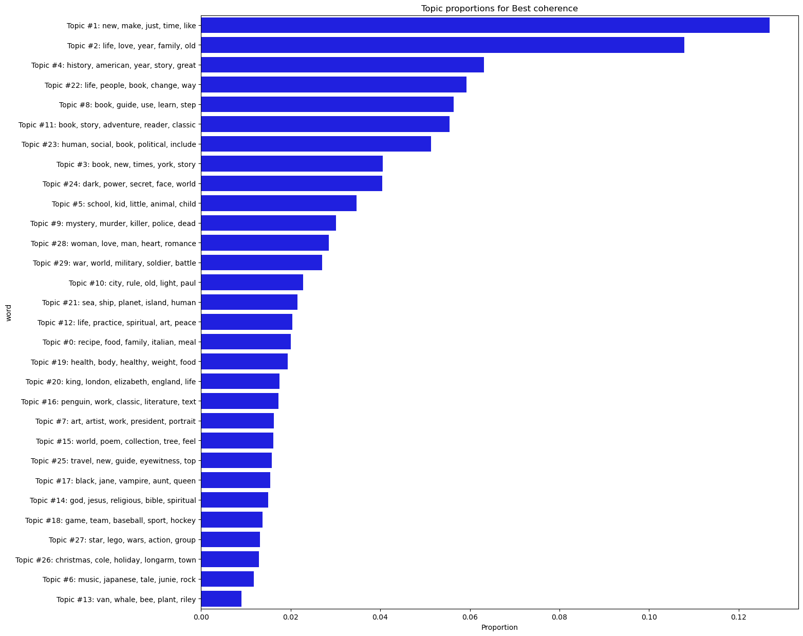
plot_topic_proportions(best_c, name = 'Best coherence')

6.5. Fine Tuning: Advanced

6.5.1. Hyperparameters: alpha and eta

The number of topics is not the only value we can set when initializing a model. LDA modeling has two key hyperparameters, which we can configure to control the nature of the topics a training run produces:

Want more details?

This StackExchange answer has a remarkably succinct summary of these two hyperparameters. Additionally, this blogpost features graphs of how changes in hyperparameters change the probability distributions in a Dirichlet space.

• Alpha: represents document-topic density. The higher the alpha, the more evenly distributed, or “symmetric,” topic proportions are in a particular document. A lower alpha means topic proportions are “asymmetric,” that is, a document will have fewer predominating topics, rather than several

• Eta: represents word-topic density. The higher the eta, the more word probabilities will be distributed evenly across a topic (specifically, this boosts the presence of low-probability words). A lower eta means word distributions are more uneven, so each topic will have less dominant words

At core, these two hyperparameters variously control specificity in models: one for the way models handle document specificity, and one for the way they handle topic specificity.

On terminology

Different LDA implementations have different names for these hyperparameters. Eta, for example, is also referred to as beta. When reading the documentation for an implementation, look for whatever term stands for the “document prior” (alpha) and the “word prior” (eta).

tomotopy has actually been setting values for alpha and eta all along. We can declare them specifically with arguments when initializing a model. Below, we boost the alpha and lessen the eta. This configuration should give us a more even distribution in topics among the documents and higher probabilities for the words in each topic. We’ll use the topic number from our best coherence model above.

ae_adjusted = tp.LDAModel(
    k = best_c.k, alpha = 1, eta = 0.001, corpus = corpus, seed = seed
)
ae_adjusted.train(iter = iters)

Let’s compare with the best coherence model.

compare = {'best coherence': best_c, 'high alpha/low eta': ae_adjusted}
for name, tm in compare.items():
    probs = []
    for topic in range(tm.k):
        scores = [s for (w, s) in tm.get_topic_words(topic, top_n = 5)]
        probs.append(scores)

    probs = np.mean(probs)
    words_per_topic = np.median(tm.get_count_by_topics())

    print(f"For the {name} model:")
    print(f"+ Median words/topic: {words_per_topic:0.0f}")
    print(f"+ Mean probablity of a topic's top-five words: {probs:0.4f}%")

For the best coherence model:
+ Median words/topic: 2652
+ Mean probablity of a topic's top-five words: 0.0175%
For the high alpha/low eta model:
+ Median words/topic: 4278
+ Mean probablity of a topic's top-five words: 0.0260%

6.5.2. Choosing hyperparameter values

In the literature about LDA modeling, researchers have suggested various ways of setting hyperparameters. For example, the authors of this paper suggest that the ideal alpha and eta values are \(\frac{50}{k}\) and 0.1, respectively (where \(k\) is the number of topics). Alternatively, you’ll often see people advocate for an approach called grid searching. This involves selecting a range of different values for the hyperparameters, permuting them, and building as many different models as it takes to go through all possible permutations.

Both approaches are valid but they don’t emphasize an important point about what our hyperparameters represent. Alpha and eta are priors, meaning they represent certain kinds of knowledge we have about our data before we even model it. In our case, we’re working with book blurbs. The generic conventions of these texts are fairly constrained, so it probably doesn’t make sense to raise our alpha values. The same might hold for a corpus of tweets collected around a small keyword set: the data collection is already a form of hyperparameter optimization. Put another way, setting hyperparameters depends on your data and your research question(s). It’s as valid to ask, “do these values give me an interpretable model?” as it is to look to perplexity and coherence scores as the sole arbiters of model quality.

Here’s an example of where the interpretability consideration matters. In the model below, we set hyperparameters to produce low perplexity and coherence scores.

optimized = tp.LDAModel(
    k = best_c.k, alpha = 5, eta = 2, corpus = corpus, seed = seed
)
optimized.train(iter = iters)
optimized_coherence = Coherence(optimized, coherence = 'c_v')

The scores look good.

print(f"Perplexity: {optimized.perplexity:0.4f}")
print(f"Coherence: {optimized_coherence.get_score():0.4f}")

Perplexity: 7354.1627
Coherence: 0.8756

But look at the topics:

for k in range(optimized.k):
    top_words(optimized, k)

Topic 0: recalcitrants (0.0001%), sculley (0.0001%), kropp (0.0001%), distort (0.0001%), sixth (0.0001%)
Topic 1: forces (0.0001%), rwanda (0.0001%), awakes (0.0001%), armada (0.0001%), inseparable (0.0001%)
Topic 2: haight (0.0001%), jung (0.0001%), youdon (0.0001%), reconstruction (0.0001%), gifts (0.0001%)
Topic 3: yugoslavia (0.0001%), mistery (0.0001%), brainiac (0.0001%), pilchuk (0.0001%), lola (0.0001%)
Topic 4: cuneiform (0.0001%), purport (0.0001%), quadratic (0.0001%), warts (0.0001%), alphabetic (0.0001%)
Topic 5: jinks (0.0001%), neuro (0.0001%), shivers (0.0001%), cull (0.0001%), beet (0.0001%)
Topic 6: new (0.0000%), life (0.0000%), book (0.0000%), world (0.0000%), story (0.0000%)
Topic 7: subdue (0.0001%), cooperative (0.0001%), heated (0.0001%), anara (0.0001%), improved (0.0001%)
Topic 8: new (0.0000%), life (0.0000%), book (0.0000%), world (0.0000%), story (0.0000%)
Topic 9: new (0.0000%), life (0.0000%), book (0.0000%), world (0.0000%), story (0.0000%)
Topic 10: corporal (0.0001%), piston (0.0001%), disembarks (0.0001%), oriented (0.0001%), introductionfrom (0.0001%)
Topic 11: new (0.0000%), life (0.0000%), book (0.0000%), world (0.0000%), story (0.0000%)
Topic 12: teroni (0.0001%), exhilarating (0.0001%), wifesanta (0.0001%), rosa (0.0001%), ragtag (0.0001%)
Topic 13: heartbreakingly (0.0001%), chances (0.0001%), vivacious (0.0001%), behindin (0.0001%), thorkellson (0.0001%)
Topic 14: new (0.0000%), life (0.0000%), book (0.0000%), world (0.0000%), story (0.0000%)
Topic 15: unfulfilled (0.0001%), cameo (0.0001%), nationis (0.0001%), paean (0.0001%), medalwinning (0.0001%)
Topic 16: new (0.0000%), life (0.0000%), book (0.0000%), world (0.0000%), story (0.0000%)
Topic 17: una (0.0001%), banda (0.0001%), coburn (0.0001%), eso (0.0001%), justamente (0.0001%)
Topic 18: possessiveness (0.0001%), dauntless (0.0001%), yearsfrom (0.0001%), goodfrom (0.0001%), meddle (0.0001%)
Topic 19: new (0.0000%), life (0.0000%), book (0.0000%), world (0.0000%), story (0.0000%)
Topic 20: underprivileged (0.0001%), widen (0.0001%), enchanting (0.0001%), rabbi (0.0001%), prop (0.0001%)
Topic 21: new (0.0000%), life (0.0000%), book (0.0000%), world (0.0000%), story (0.0000%)
Topic 22: new (0.0000%), life (0.0000%), book (0.0000%), world (0.0000%), story (0.0000%)
Topic 23: del (0.0001%), que (0.0001%), elendel (0.0001%), más (0.0001%), mistborn (0.0001%)
Topic 24: sneezing (0.0001%), haynes (0.0001%), choucroute (0.0001%), tanksincludes (0.0001%), literaturelabeled (0.0001%)
Topic 25: boomer (0.0001%), transformationfor (0.0001%), cosimo (0.0001%), nergal (0.0001%), coerce (0.0001%)
Topic 26: new (0.0000%), life (0.0000%), book (0.0000%), world (0.0000%), story (0.0000%)
Topic 27: new (0.0000%), life (0.0000%), book (0.0000%), world (0.0000%), story (0.0000%)
Topic 28: new (0.0056%), life (0.0052%), book (0.0050%), world (0.0037%), story (0.0035%)
Topic 29: josephus (0.0001%), employees (0.0001%), snowbound (0.0001%), chaffino (0.0001%), hatches (0.0001%)

And the proportions:

plot_topic_proportions(optimized, name = 'Hyperoptimized')

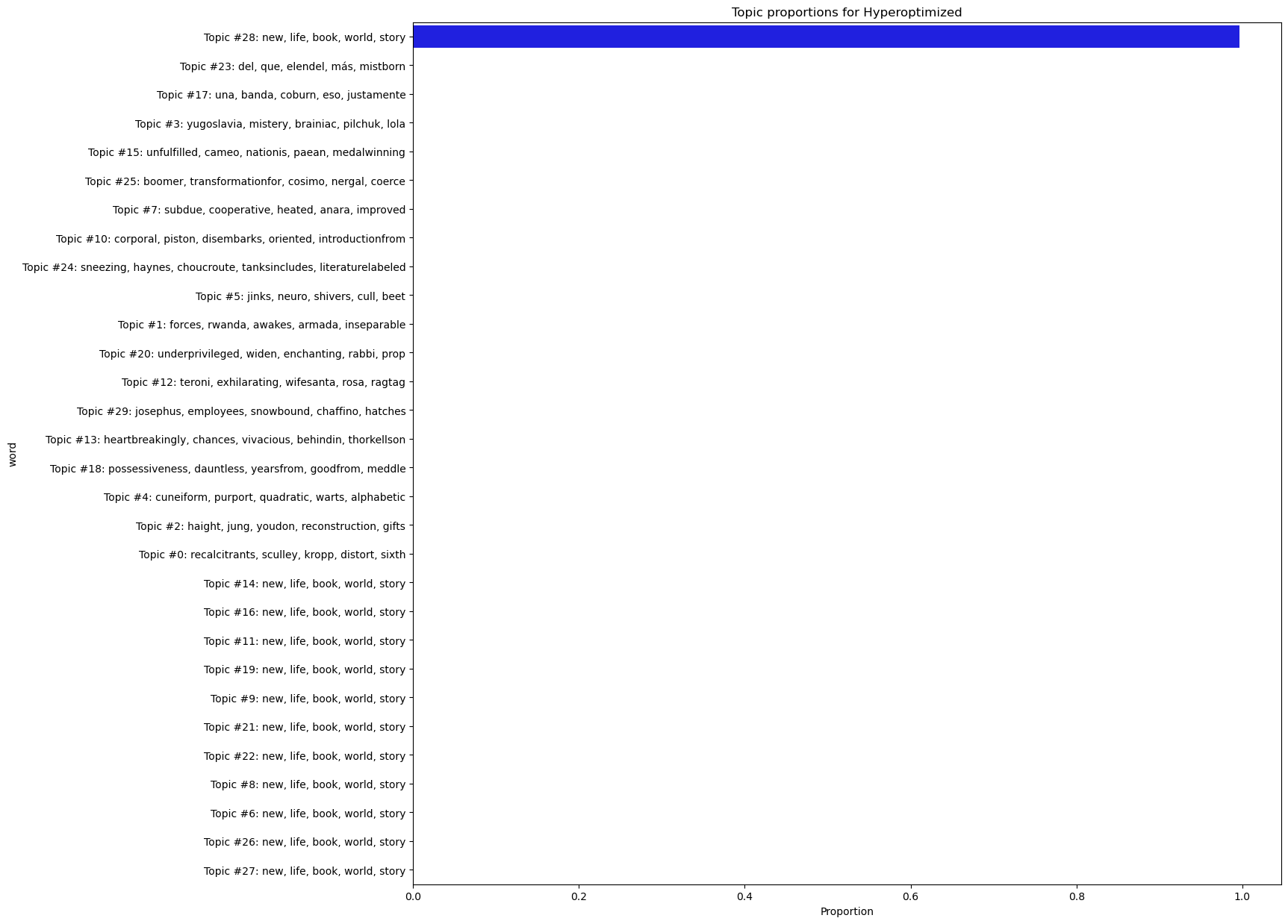
The top words are incoherent and one topic all but completely dominates the topic distribution.

The challenge of setting hyperparameters, then, is that it’s a balancing act. In light of the above output, for example, you might decide to favor interpretability above everything else. But doing so can lead to overfitting. Hence the balancing act: the whole process of fine tuning involves incorporating a number of different considerations (and compromises!) that, at the end of the day, should work in the service of your research question.

6.5.3. Final configuration

To return to the question of our own corpus, here are the best topic number/hyperparameter configuration from a grid search run:

grid_df = pd.read_csv(indir.joinpath("grid_search_results.csv"), index_col = 0)
grid_df.sort_values('coherence', ascending = False, inplace = True)
grid_df.head(10)

	n_topics	alpha	eta	perplexity	coherence
315	29	0.100	0.0150	10190.744366	0.726677
335	30	0.125	0.0150	10101.535785	0.723886
323	30	0.050	0.0150	10248.757358	0.721783
318	29	0.125	0.0125	10449.013502	0.720463
310	29	0.075	0.0125	10630.975052	0.719463
326	30	0.075	0.0125	10241.915592	0.718477
330	30	0.100	0.0125	10304.032934	0.717663
275	27	0.050	0.0150	10222.881381	0.716541
319	29	0.125	0.0150	10266.766973	0.714951
311	29	0.075	0.0150	10229.393637	0.712904

If you look closely at the scores, you’ll see that they’re all very close to one another; any one of these options would make for a good model. The perplexity is a bit high, but the coherence scores look good and the topic numbers produce a nice spread of topics. Past testing has shown that the following configuration makes for a particularly good – which is to say, interpretable – one:

tuned = tp.LDAModel(
    k = 29, alpha = 0.1, eta = 0.015, corpus = corpus, seed = seed
)
tuned.train(iter = iters)
tuned_coherence = Coherence(tuned, coherence = 'c_v')

Our metrics:

print(f"Perplexity: {tuned.perplexity:0.4f}")
print(f"Coherence: {tuned_coherence.get_score():0.4f}")

Perplexity: 10170.1982
Coherence: 0.7075

Our topics:

for k in range(tuned.k):
    top_words(tuned, k)

Topic 0: war (0.0457%), history (0.0138%), soldier (0.0124%), military (0.0108%), line (0.0087%)
Topic 1: new (0.0184%), make (0.0177%), just (0.0156%), like (0.0138%), time (0.0129%)
Topic 2: child (0.0276%), mother (0.0263%), school (0.0253%), parent (0.0214%), family (0.0201%)
Topic 3: adventure (0.0180%), cat (0.0176%), love (0.0156%), tale (0.0145%), animal (0.0121%)
Topic 4: music (0.0202%), american (0.0143%), song (0.0123%), star (0.0119%), film (0.0115%)
Topic 5: team (0.0179%), money (0.0157%), game (0.0148%), sport (0.0139%), financial (0.0125%)
Topic 6: book (0.0456%), child (0.0188%), reader (0.0157%), little (0.0146%), young (0.0142%)
Topic 7: christmas (0.0259%), horse (0.0173%), town (0.0147%), cole (0.0125%), family (0.0117%)
Topic 8: murder (0.0272%), mystery (0.0225%), killer (0.0139%), crime (0.0136%), police (0.0130%)
Topic 9: band (0.0132%), aunt (0.0108%), amy (0.0102%), junie (0.0096%), jones (0.0096%)
Topic 10: political (0.0270%), america (0.0139%), states (0.0114%), united (0.0103%), politics (0.0095%)
Topic 11: secret (0.0143%), world (0.0122%), new (0.0103%), human (0.0088%), power (0.0085%)
Topic 12: life (0.0261%), story (0.0246%), year (0.0195%), world (0.0167%), family (0.0105%)
Topic 13: recipe (0.0277%), food (0.0258%), italian (0.0117%), family (0.0104%), meal (0.0095%)
Topic 14: star (0.0240%), universe (0.0146%), planet (0.0142%), lego (0.0138%), wars (0.0134%)
Topic 15: work (0.0174%), penguin (0.0171%), classic (0.0156%), introduction (0.0147%), english (0.0144%)
Topic 16: guide (0.0305%), travel (0.0138%), new (0.0134%), include (0.0128%), top (0.0121%)
Topic 17: comic (0.0179%), volume (0.0124%), tale (0.0115%), sword (0.0107%), adventure (0.0098%)
Topic 18: york (0.0554%), new (0.0526%), times (0.0514%), book (0.0283%), author (0.0269%)
Topic 19: guide (0.0175%), help (0.0136%), learn (0.0109%), health (0.0107%), program (0.0101%)
Topic 20: novel (0.0231%), reader (0.0165%), character (0.0142%), story (0.0128%), author (0.0123%)
Topic 21: van (0.0108%), ellie (0.0101%), landscape (0.0074%), riley (0.0068%), quinn (0.0068%)
Topic 22: book (0.0189%), work (0.0101%), life (0.0098%), world (0.0092%), people (0.0091%)
Topic 23: art (0.0411%), artist (0.0237%), step (0.0227%), use (0.0167%), create (0.0157%)
Topic 24: sea (0.0213%), ship (0.0159%), island (0.0101%), sam (0.0093%), crew (0.0093%)
Topic 25: woman (0.0437%), love (0.0358%), life (0.0225%), husband (0.0152%), passion (0.0130%)
Topic 26: century (0.0183%), king (0.0179%), history (0.0171%), london (0.0149%), great (0.0086%)
Topic 27: vampire (0.0156%), dead (0.0139%), hunter (0.0110%), black (0.0110%), queen (0.0101%)
Topic 28: god (0.0339%), life (0.0277%), spiritual (0.0215%), practice (0.0177%), book (0.0143%)

Our proportions:

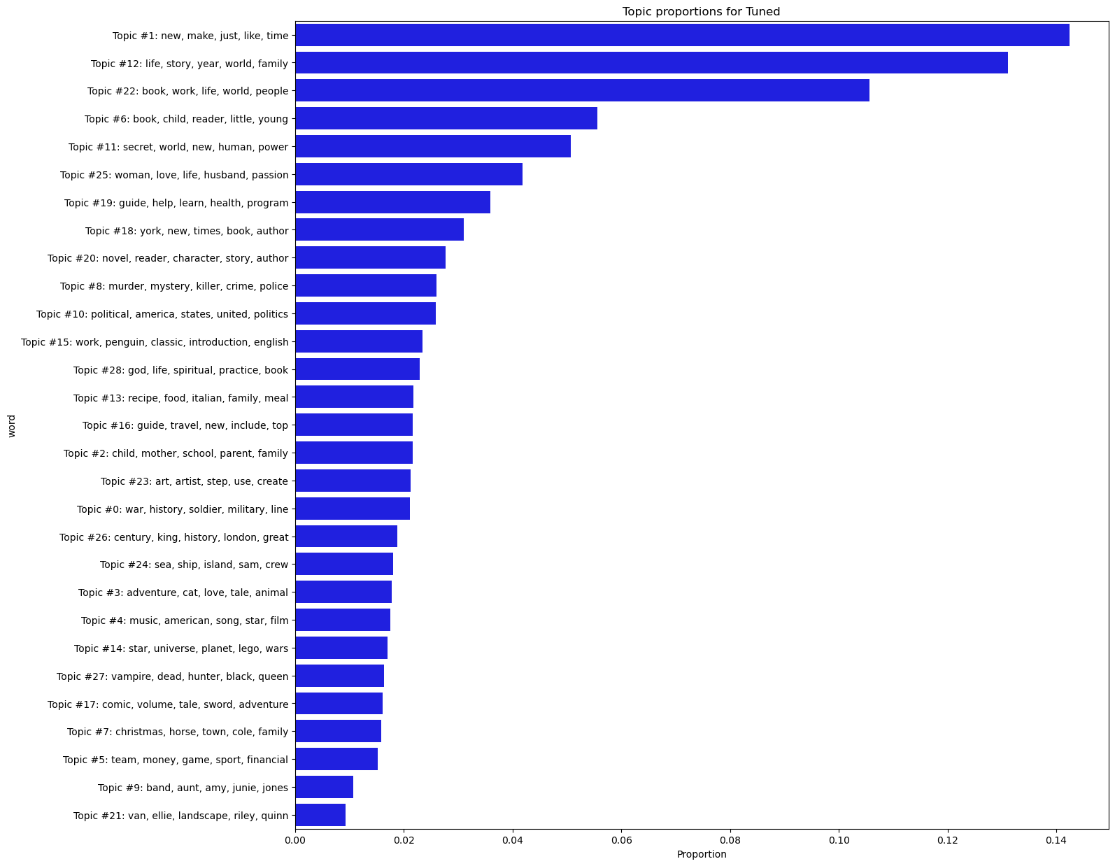
plot_topic_proportions(tuned, name = 'Tuned')

6.6. Model Exploration

Topic proportions and top words are all helpful, but there are other ways to dig more deeply into a model. This final section will show you a few examples of this.

First, let’s rebuild a theta matrix from the fine-tuned model. Remember that a theta is a document-topic matrix, where each cell is a probability score for a document’s association with a particular topic.

theta = get_theta(tuned, manifest['title'])

We’ll also make a quick set of labels for our topics, which list the top five words for each one.

labels = [format_top_words(tuned, k) for k in range(tuned.k)]

A heatmap is a natural fit for inspecting the probability distributions of theta.

n_samples = 20
blurb_set = manifest['title'].sample(n_samples)
sub_theta = theta[theta.index.isin(blurb_set)]

fig, ax = plt.subplots(figsize = (15, 8))
g = sns.heatmap(sub_theta, linewidths = 1, cmap = 'Blues', ax = ax)
g.set(xlabel = 'Topic', ylabel = 'Title', xticklabels = labels)
ax.xaxis.set_label_position('top')
ax.xaxis.tick_top()
plt.xticks(rotation = 30, ha = 'left')
plt.tight_layout();

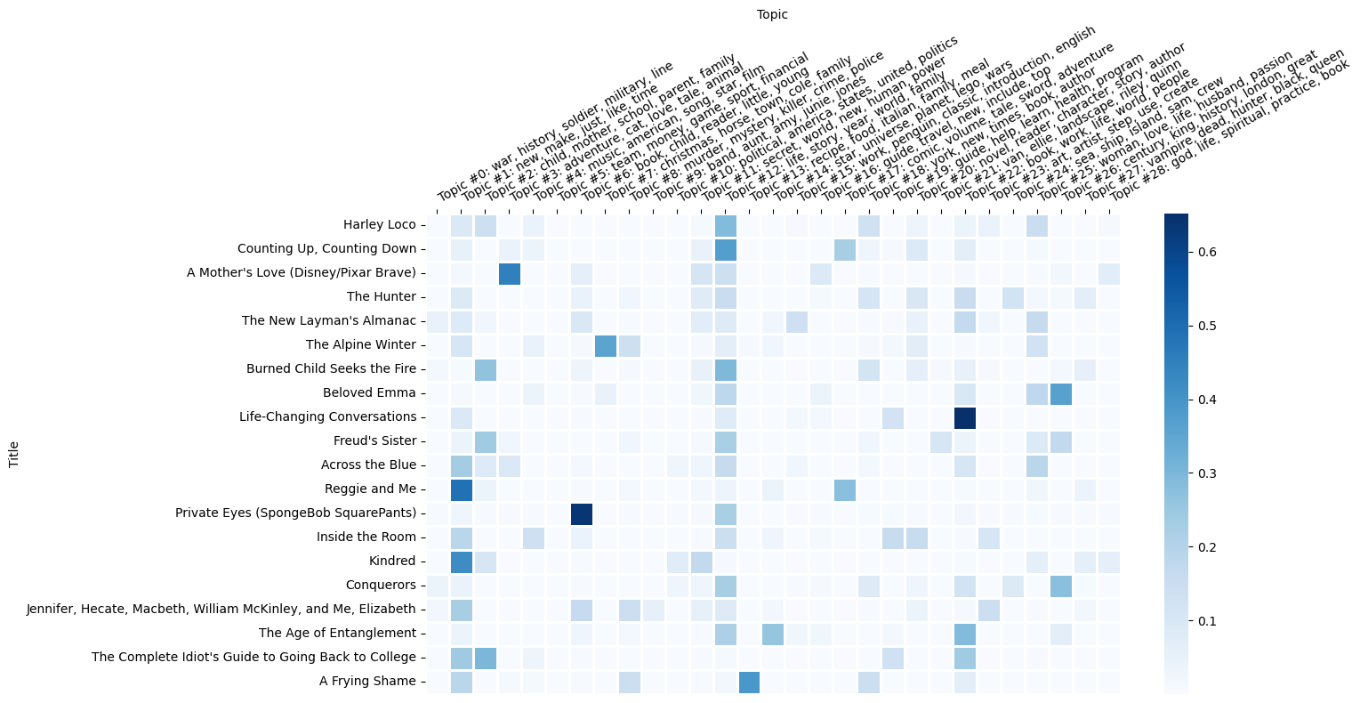
Topic 15 appears to be about the classics. What kind of titles have a particularly high association with this topic?

def doc_topic_associations(theta, manifest, k):
    """Find highly associated documents from a manifest with a topic."""
    topk = theta.loc[theta.idxmax(axis = 1) == k, k]
    associated = manifest[manifest['title'].isin(topk.index)].copy()
    associated.loc[:, f'{k}_score'] = topk.values

    return associated[['author', 'title', 'genre', f'{k}_score']]

k15 = doc_topic_associations(theta, manifest, 15)
k15.head(15)

	author	title	genre	15_score
1	Horatio Alger	Ragged Dick and Struggling Upward	Classics	0.510900
66	Chris Carter, Roy Thomas, Glenn Morgan, James ...	X-Files Classics: Season 1 Volume 1	Fiction	0.344544
146	Marge Piercy	The Art of Blessing the Day	Poetry	0.174064
258	Chretien de Troyes	Arthurian Romances	Classics	0.731107
271	Various	American Science Fiction: Nine Classic Novels ...	Fiction	0.350466
275	Nicola Sacco, Bartolomeo Vanzetti	The Letters of Sacco and Vanzetti	Classics	0.588130
412	Michel de Montaigne	The Essays	Classics	0.291393
443	David Goodis	The Burglar	Fiction	0.221486
464	Frances Hodgson Burnett	A Little Princess	Classics	0.246585
480	Laura Ingalls Wilder	Laura Ingalls Wilder: The Little House Books V...	Fiction	0.358375
485	Brooks Haxton	They Lift Their Wings to Cry	Classics	0.191476
595	Mary Boykin Chesnut	Mary Chesnut's Diary	Classics	0.522240
601	Kenneth Grahame	The Wind in the Willows	Classics	0.633616
621	Harriet Jacobs	Incidents in the Life of a Slave Girl	Classics	0.573353
631	Richard E. Kim	The Martyred	Classics	0.425864

Certain topics seem to map very nicely onto particular book genres. Here are some titles associated with topic 13, which is about recipes.

k13 = doc_topic_associations(theta, manifest, 13)
k13.head(15)

	author	title	genre	13_score
8	Adele Yellin, Kevin West	The Grand Central Market Cookbook	Nonfiction	0.432363
17	Gene Daoust, Joyce Daoust	The Formula	Nonfiction	0.352713
188	Lilach German	Cookies, Cookies & More Cookies!	Nonfiction	0.382768
233	Katharine Ibbs	DK Children's Cookbook	Nonfiction	0.455814
279	Christina Orchid	Christina's Cookbook	Nonfiction	0.421846
327	Nicola Graimes	The Low-Sugar Cookbook	Nonfiction	0.439704
368	Sara Deseran, Joe Hargrave, Antelmo Faria, Mik...	Tacolicious	Nonfiction	0.663644
395	Kendra Bailey Morris	The Southern Slow Cooker	Nonfiction	0.509477
452	Carmen Posadas	Little Indiscretions	Fiction	0.201231
459	Suvir Saran, Stephanie Lyness	Indian Home Cooking	Nonfiction	0.683412
462	Helene Siegel	Totally Salmon Cookbook	Nonfiction	0.653585
549	Carly de Castro, Hedi Gores, Hayden Slater	Juice	Nonfiction	0.406312
578	Hi Soo Shin Hepinstall	Growing up in a Korean Kitchen	Nonfiction	0.379062
612	Maria del Mar Sacasa	Winter Cocktails	Nonfiction	0.438557
620	Frank Pellegrino	Rao's Cookbook	Nonfiction	0.541190

Topic 2 appears to be about girlhood.

k2 = doc_topic_associations(theta, manifest, 2)
k2.head(15)

	author	title	genre	2_score
9	Liz Curtis Higgs	Thorn in My Heart	Fiction	0.306729
90	Paul D. White, Ron Arias	White's Rules	Nonfiction	0.260193
153	Liz Curtis Higgs	Grace in Thine Eyes	Fiction	0.305969
278	Julianna Margulies, Paul Margulies	Three Magic Balloons	Children’s Books	0.289717
328	John Ramsey Miller	The Last Family	Fiction	0.392691
382	Val Brelinski	The Girl Who Slept with God	Fiction	0.274784
416	Sarah Henstra	Mad Miss Mimic	Teen & Young Adult	0.216246
678	Leigh Stein	The Fallback Plan	Fiction	0.363485
698	Suzanne Fisher Staples	The House of Djinn	Teen & Young Adult	0.305969
718	Goce Smilevski	Freud's Sister	Fiction	0.241625
763	Edd Doerr	The Case Against School Vouchers	Nonfiction	0.276409
897	Adolf Schroder	The Game of Cards	Fiction	0.294001
921	Bobby Henderson	The Gospel of the Flying Spaghetti Monster	Classics	0.227076
942	Manuela Monari	Zero Kisses for Me	Children’s Books	0.360254
1142	Emily Bazelon	Sticks and Stones	Nonfiction	0.257467

Though there are some perplexing titles listed here. What’s The Gospel of the Flying Spaghetti Monster doing here? The Case Against School Vouchers is similarly odd, though maybe it’s a sensible fit given what we might expect from shared vocabulary. Topic models, remember, are ultimately counting word co-occurrences, not the different semantic valences of a word, or tone, style, etc. It’s up to us to parse the latter kinds of things.

To do so, it’s helpful to examine the overall similarities and differences between topics, much in the way we projected our documents into a vector space in the previous chapter. We’ll prepare the code to do something similar here but will save the final result for a separate webpage. Below, we produce the following:

• A topic-term distribution matrix (word probabilities for each topic)

• The lengths of every blurb

• A list of the corpus vocabulary

• The corresponding frequency counts for the corpus vocabulary

Once we’ve made these, we’ll prepare our visualization data with a package called pyLDAvis and save it.

topic_terms = np.stack([tuned.get_topic_word_dist(k) for k in range(tuned.k)])
doc_lengths = np.array([len(doc.words) for doc in tuned.docs])
vocab = list(tuned.used_vocabs)
term_frequency = tuned.used_vocab_freq

vis = pyLDAvis.prepare(
    topic_terms, theta.values, doc_lengths, vocab, term_frequency,
    start_index = 0, sort_topics = False
)

outdir = indir.joinpath("output/topic_model_plot.html")
pyLDAvis.save_html(vis, outdir.as_posix())

With that done, we’ve finished our initial work with topic models. The resultant visualization of the above is available here. It’s a scatter plot that represents topic similarity; the size of each topic circle corresponds to that topic’s proportion in the model. Explore it some and see what you find!