4. Corpus Analytics

This chapter moves from an individual text to a collection of texts, or a corpus. While computational methods may lead us to discover interesting things about texts in isolation, they’re often at their best when we use them to study texts at scale. We’ll do just that in this chapter: below, you’ll learn how to compile texts into a corpus and generate several metrics about these texts. Doing so will enable us to observe similarities/differences across the corpus at scale.

We’ll also leave Frankenstein behind and turn instead to Melanie Walsh’s collection of ~380 obituaries from the New York Times. “Obituary subjects,” writes Walsh, “include academics, military generals, artists, athletes, activities, politicians, and businesspeople – such as Ada Lovelace, Ulysses Grant, Marilyn Monroe, Virginia Woolf, Jackie Robinson, Marsha P. Johnson, Cesar Chavez, John F. Kennedy, Ray Kroc, and many more.”

Learning Objectives

By the end of this chapter, you will be able to:

• Compile texts into a corpus

• Use a document-term matrix to represent relationships in the corpus

• Generate metrics about texts in a corpus

• Explain the difference between raw term metrics and weighted term scoring

4.1. Preliminaries

4.1.1. Setup

Before we get into corpus construction, let’s load the libraries we’ll be using throughout the chapter.

from pathlib import Path
import re
import numpy as np
import pandas as pd
from sklearn.feature_extraction.text import CountVectorizer, TfidfVectorizer
import matplotlib.pyplot as plt
import seaborn as sns

Initialize a path to the data directory as well.

indir = Path("data/session_two")

4.1.2. File manifest

We’ll also use a file manifest for this chapter. It contains metadata about the corpus, and we’ll also use it to keep track of our corpus construction.

manifest = pd.read_csv(indir.joinpath("manifest.csv"), index_col = 0)
manifest.info()

<class 'pandas.core.frame.DataFrame'>
Index: 379 entries, 0 to 378
Data columns (total 3 columns):
 #   Column     Non-Null Count  Dtype 
---  ------     --------------  ----- 
 0   name       379 non-null    object
 1   year       379 non-null    int64 
 2   file_name  379 non-null    object
dtypes: int64(1), object(2)
memory usage: 11.8+ KB

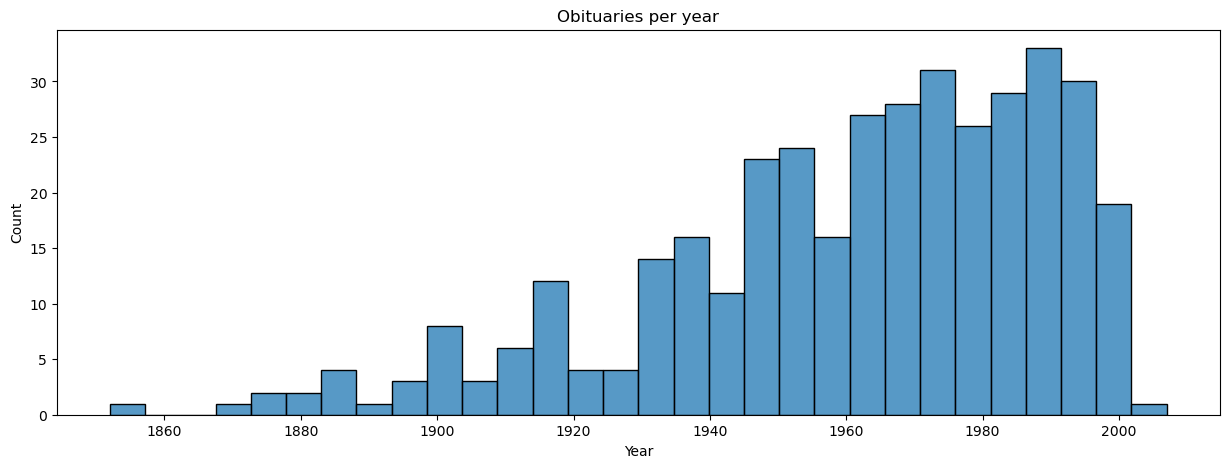
A brief plot of the years covered:

fig, ax = plt.subplots(figsize = (15, 5))
g = sns.histplot(x = 'year', bins = 30, data = manifest, ax = ax)
g.set(title = 'Obituaries per year', xlabel = 'Year', ylabel = 'Count');

Tip

Using a metadata sheet like this is a good habit to develop. Use it as a common reference point for any processes you run on your data, and you’ll metigate major headaches stemming from undocumented projects. For more on this, see the DataLab’s workshop on project organization and data documentation.

4.2. Compiling a Corpus

The obituaries are stored as individual files, which we need to load into memory and combine into a corpus. Because cleaning can be labor- and time-intensive, these texts have already been cleaned (lemmatization included). You can find the script that performed this cleaning here.

Corpus compilation is fairly straightforward: we’ll load everything in a for loop. But the order of these texts is important, and this is where the file manifest comes in. Using the manifest, we’ll load the texts in the order provided by the file_name column. Doing so ensures that the first index (0) of our corpus corresponds to the first text, the second index (1) to the second, and so on.

corpus = []
for title in manifest.index:
    fname = manifest.loc[title, 'file_name']
    path = indir.joinpath(f"input/{fname}")
    with path.open('r') as fin:
        corpus.append(fin.read())

Let’s double-check that this has worked. First, we run an assertion to ensure that the number of texts match the number of entries in our manifest.

assert len(corpus) == len(manifest), "Length's don't match!"

Second, let’s inspect a few pieces of the texts.

for idx in range(3):
    print(corpus[idx][:25])

gifted mathematician reco
october obituary gen robe
august obituary andrew jo

Looks great!

4.3. The Document-Term Matrix

Before we switch into data exploration mode, we’ll perform one last formatting process on our corpus. Remember from the last chapter that much of text analytics relies on counts and contexts. As with Frankenstein, one thing we want to do is tally up all the words in each text. That produces one kind of context – or rather, a few hundred different contexts: one for each file we’ve loaded. But we also compiled these files into a corpus, the analysis of which requires a different kind of context: a single one for all the texts. That is, we need a way to relate texts to each other, instead of only tracking word values inside a single text.

To do so, we’ll build a document-term matrix, or DTM. A DTM is a matrix that contains the frequencies of all terms in a corpus. Every row in this matrix corresponds to a text, while every column corresponds to a term. For a given text, we count the number of times that term appears and enter that number in the column in question. We do this even if the count is zero; key to the way a DTM works is that it represents corpus-wide relationships between texts, so it matters if a text does or doesn’t contain a term.

Here’s a toy example. Imagine three documents:

1. “I like cats. Do you?”

2. “I only like dogs. And you?”

3. “I like cats and dogs.”

Transforming them into a DTM would yield:

example = [
    [1, 0, 1, 1, 0, 0, 1, 1],
    [1, 1, 1, 0, 1, 1, 0, 1],
    [1, 0, 1, 1, 1, 1, 0, 0]
]
names = ['D1', 'D2', 'D3']
terms = ['i', 'only', 'like', 'cats', 'and', 'dogs', 'do', 'you']
example_dtm = pd.DataFrame(example, columns = terms, index = names)
example_dtm

	i	only	like	cats	and	dogs	do	you
D1	1	0	1	1	0	0	1	1
D2	1	1	1	0	1	1	0	1
D3	1	0	1	1	1	1	0	0

Representing texts in this way is incredibly useful because it enables us to discern similarities/differences in our corpus with ease. For example, all of the above documents contain the words “i” and “like.” Given that, if we wanted to know what makes each document unique, we could ignore those two words and focus on the rest of the values.

Now imagine doing this for thousands of words. What patterns might emerge?

More on this

CountVectorizer accepts several arguments that modify its base functionality, including arguments for applying some text cleaning steps. We won’t use any of these arguments because we’ve cleaned our texts already, but you can learn more about them here.

The scikit-learn library makes generating a DTM very easy. All we need to do is initialize a CountVectorizer and fit it to our corpus. This does two things: 1) it produces a series of different attributes that are useful for corpus exploration; 2) it generates our DTM.

count_vectorizer = CountVectorizer()
vectorized = count_vectorizer.fit_transform(corpus)

print("Shape of our DTM:", vectorized.shape)

Shape of our DTM: (379, 31165)

CountVectorizer returns a sparse matrix, or a matrix comprised mostly of zeros. This matrix is formatted to be highly memory efficient, which is useful when dealing with big datasets, but it’s not very accessible for data exploration. Since our corpus is relatively small, we’ll convert this sparse matrix to a pandas DataFrame.

We will also call our vectorizer’s .get_feature_names_out() method. This generates an array of all the tokens from all the obituaries. The order of this array corresponds to the order of the DTM’s columns. Accordingly, we assign this array to the column names of our DTM. Finally, we assign the name column values from our manifest to the index of our DTM.

dtm = pd.DataFrame(
    vectorized.toarray(),
    columns = count_vectorizer.get_feature_names_out(),
    index = manifest['name']
)

4.4. Raw Metrics

With the DTM made, it’s time to use it to generate some metrics about each text in the corpus. We use pandas data manipulations in conjunction with NumPy to do so; the function below will make plots for us.

def plot_metrics(data, col, title = '', xlabel = ''):
    """Plot metrics with a histogram."""
    fig, ax = plt.subplots(figsize = (15, 5))
    g = sns.histplot(x = col, data = data)
    g.set(title = title, xlabel = xlabel, ylabel = 'Count');

4.4.1. Documents

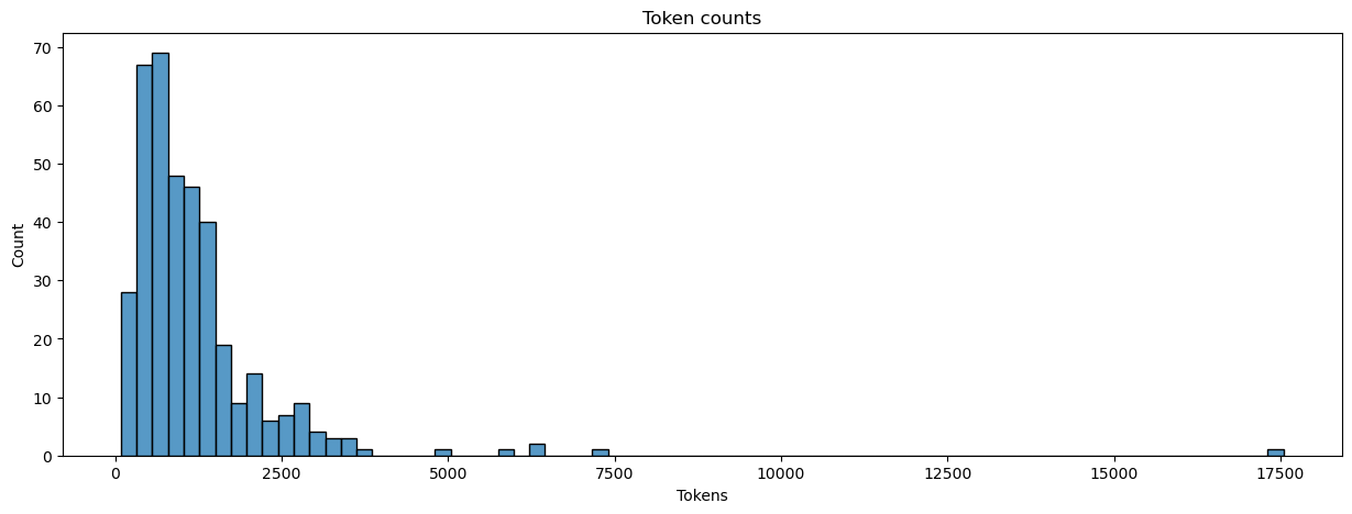
Here’s an easy one: let’s count the number of tokens in each text and assign the result to a new column in our manifest.

manifest.loc[:, 'num_tokens'] = dtm.apply(sum, axis = 1).values
plot_metrics(manifest, 'num_tokens', title = 'Token counts', xlabel = 'Tokens')

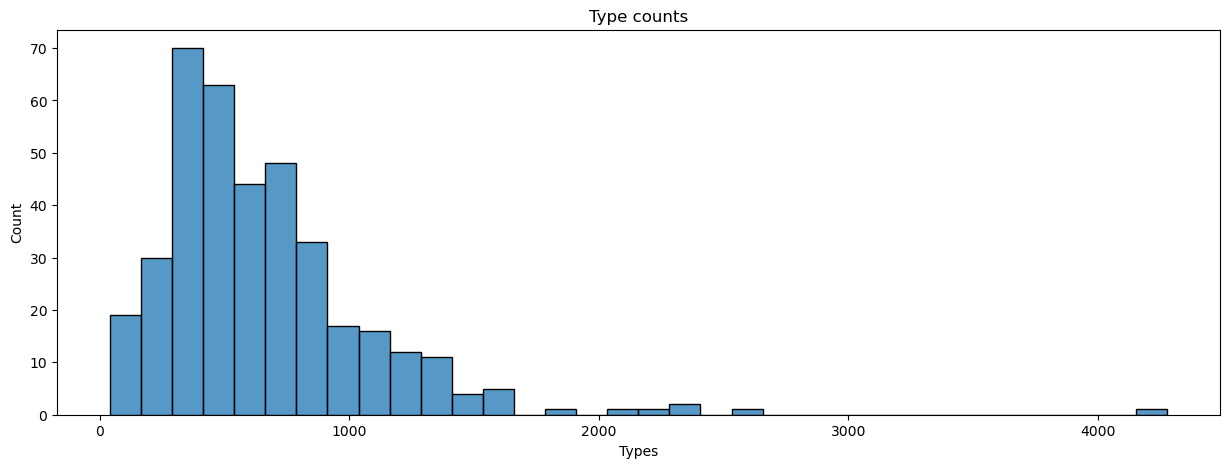
We can also count the number of unique words, or types, in each text. Types correspond to a text’s vocabulary, whereas tokens correspond to the amount of each of those types.

manifest.loc[:, 'num_types'] = dtm.apply(np.count_nonzero, axis = 1).values
plot_metrics(manifest, 'num_types', title = 'Type counts', xlabel = 'Types')

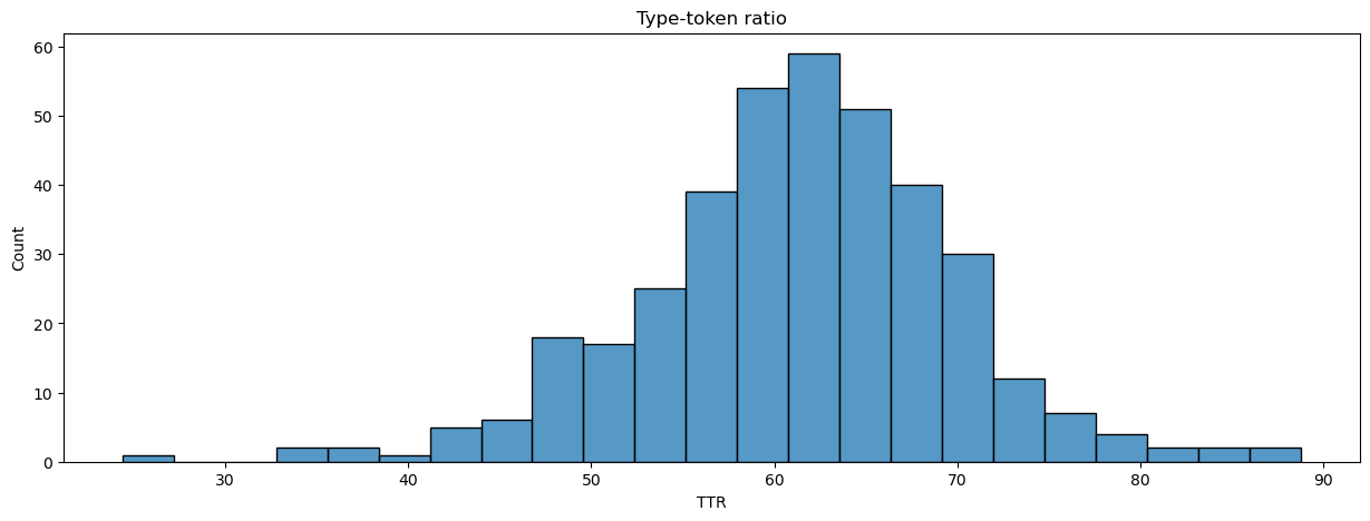
We can use tokens and types to generate a metric of lexical diversity. There are a few such measures. We’ll use the type-token ratio (TTR), which measures how much the vocabulary of a text varies over its tokens. It’s a simple metric: divide the number of types by the total number of tokens in a text and normalize the result. A text with a TTR of 100, for example, would never repeat a word.

manifest.loc[:, 'TTR'] = (manifest['num_types'] / manifest['num_tokens']) * 100
plot_metrics(manifest, 'TTR', title = 'Type-token ratio', xlabel = 'TTR')

What are examples of texts that typify the low, medium, and high range of these metrics? The function below will pull up examples for each range.

Code explanation

This function uses qcut() to bin metric values into a set of categories. The output of qcut() is a Series. We match the index of this Series to our DataFrame, pull out a random name from each bin, and print it.

def show_examples(data, metric, labels = ['low', 'medium', 'high']):
    cuts = pd.qcut(data[metric], len(labels), labels = labels)
    for label in labels:
        idxes = cuts[cuts==label].index
        ex = data[data.index.isin(idxes)].sample()
        print(f"+ {label}: {ex['name'].item()} ({ex[metric].item():0.2f})")

for metric in ('num_tokens', 'num_types', 'TTR'):
    print("Examples for", metric)
    show_examples(manifest, metric)
    print("\n")

Examples for num_tokens
+ low: Walker Evans (523.00)
+ medium: Eugene O Neill (1128.00)
+ high: Orson Welles (1484.00)


Examples for num_types
+ low: Yuri Gagarin (332.00)
+ medium: Frank Capra (612.00)
+ high: Jane Addams (744.00)


Examples for TTR
+ low: Harry S Truman (43.00)
+ medium: Fred W Friendly (60.06)
+ high: Edna St V Millay (68.75)

4.4.2. Terms

Let’s move on to terms. Here are the top-five most frequent terms in the corpus:

summed = pd.DataFrame(dtm.sum(), columns = ('count', ))
summed.sort_values('count', ascending = False, inplace = True)
summed.head(5)

	count
year	3929
say	3009
new	2350
make	2258
time	2191

And here are the bottom five:

summed.tail(5)

	count
kappler	1
kapuskasing	1
karamchand	1
karat	1
zwilich	1

Though there are likely to be quite a few one-count terms. We refer to them as hapax legomena (Greek for “only said once”). How many are in our corpus altogether?

hapaxes = summed[summed['count'] == 1]
print(f"{len(hapaxes)} hapaxes ({len(hapaxes) / len(dtm.T) * 100:0.2f}%)")

12399 hapaxes (39.79%)

If we plot our term counts, we’ll see a familiar pattern: our term distribution is Zipfian.

fig, ax = plt.subplots(figsize = (15, 5))
g = sns.lineplot(x = summed.index, y = 'count', data = summed)
g.set(title = 'Term distribution', xlabel = 'Terms', xticks = []);

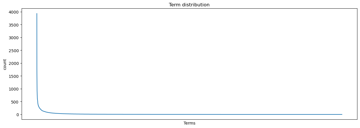
This distribution has a few consequences. It suggests, for example, that we might have more cleaning to do in terms of our stopwords: perhaps our list hasn’t accounted for some words, and if we don’t remove them, we might have trouble identifying more unique aspects of each text in our corpus. But on the other hand, all of those hapaxes are a little too unique: one option would be to drop them entirely.

But dropping our hapaxes might lose out on some specificity in our texts. And there are some highly frequent words that we want to retain (“year” and “make” for example). So what to do? How can we reduce the influence of highly frequent terms without removing them, and how can we take into account rare words at the same time?

4.5. Weighted Metrics

The answer is to weight our terms, doing so in a way that lessens the impact of high frequency terms and boosts that of rare ones. The most popular weighting method is tf-idf, or term frequency–inverse document frequency, scoring. A tf-idf score is a measure of term specificity in the context of a given document. It is the product of a term’s frequency in that document and the number of documents in which that term appears. By offsetting terms that appear across many documents, tf-idf pushes down the scores of common terms and boosts the scores of rarer ones.

A tf-idf score is expressed

The idf score

We calculate the inverse document frequency score with

\[ idf_{i} = log(\frac{n}{df_{i}}) \]

Where the score for term \(i\) is the log of the total number of total documents (\(n\)) over the number of documents that contain \(i\).

\[ score_{ij} = tf_{ij} \cdot idf_{i} \]

Where, for term \(i\) and document \(j\), the score is the term frequency (\(tf_{ij}\)) for \(i\) multiplied by its inverse document frequency (\(idf_{i}\)). The higher the score, the more specific a term is to a given document.

We don’t need to implement any of this math ourselves. scikit-learn has a TfidfVectorizer object, which works just like CountVectorizer, but instead of producing a DTM of raw term counts, it produces one with tf-idf scores.

tfidf_vectorizer = TfidfVectorizer()
vectorized_tfidf = tfidf_vectorizer.fit_transform(corpus)
tfidf = pd.DataFrame(
    vectorized_tfidf.toarray(),
    columns = tfidf_vectorizer.get_feature_names_out(),
    index = manifest['name']
)

To see the difference tf-idf scores make, let’s compare raw counts and tf-idf scores for three texts.

def counts_vs_tfidf(dtm, tfidf, idx, n_terms = 10):
    """Compare raw document counts with tf-idf scores."""
    c = dtm.loc[idx].nlargest(n_terms)
    t = tfidf.loc[idx].nlargest(n_terms)
    df = pd.DataFrame({
        'count_term': c.index, 'count': c.values,
        'tfidf_term': t.index, 'tfidf': t.values
    })

    return df

for name in manifest['name'].sample(3):
    comparison = counts_vs_tfidf(dtm, tfidf, name)
    print("Person:", name)
    display(comparison)

Person: Geronimo

	count_term	count	tfidf_term	tfidf
0	geronimo	13	geronimo	0.542158
1	chief	12	miles	0.277617
2	old	10	lawton	0.277554
3	year	10	fort	0.199686
4	gen	8	gen	0.187141
5	miles	8	chief	0.182307
6	fort	7	indian	0.178554
7	indian	7	crook	0.152230
8	lawton	7	apache	0.125113
9	men	7	apaches	0.125113

Person: Ferdinand Marcos

	count_term	count	tfidf_term	tfidf
0	marcos	39	marcos	0.886187
1	say	20	tiwanak	0.170100
2	family	8	aquino	0.145800
3	body	7	philippines	0.106012
4	mrs	7	say	0.084641
5	tiwanak	7	kidney	0.077714
6	aquino	6	aruiza	0.072900
7	death	6	ferdinand	0.060080
8	die	6	body	0.056858
9	philippines	6	dialysis	0.048600

Person: Coleman Hawkins

	count_term	count	tfidf_term	tfidf
0	hawkins	28	hawkins	0.690168
1	play	18	jazz	0.244983
2	jazz	12	saxophone	0.211016
3	style	9	saxophonist	0.184639
4	saxophone	8	play	0.155607
5	use	8	tenor	0.150996
6	musician	7	trumpet	0.133719
7	saxophonist	7	musician	0.123503
8	develop	6	style	0.108070
9	make	6	henderson	0.100664

There are a few things to note here. First, names often have the largest value, regardless of our metric. This makes intuitive sense for our corpus: we’re examining obituaries, where the sole subject of each text may be referred to many times. A tf-idf score will actually reinforce this effect, since names are often specific to the obituary. We can see this especially from the shifts taht take place in the rest of the rankings. Whereas raw counts will often refer to more general nouns and verbs, tf-idf scores home in on other people with whom the present person might’ve been associated, places that person might’ve visited, and even things that particular person is known for. Broadly speaking, tf-idf scores give us a more situated sense of the person in question.

To see this in more detail, let’s look at a single obituary in the context of the entire corpus. We’ll compare the raw counts and tf-idf scores of this obituary to the mean counts and scores of the corpus.

kahlo = counts_vs_tfidf(dtm, tfidf, 'Frida Kahlo', 15)
kahlo.loc[:, 'corpus_count'] = dtm[kahlo['count_term']].mean().values
kahlo.loc[:, 'corpus_tfidf'] = tfidf[kahlo['tfidf_term']].mean().values

cols = ['count_term', 'count', 'corpus_count', 'tfidf_term', 'tfidf', 'corpus_tfidf']
kahlo = kahlo[cols]
kahlo

	count_term	count	corpus_count	tfidf_term	tfidf	corpus_tfidf
0	artist	4	0.575198	frida	0.374507	0.000988
1	diego	3	0.047493	kahlo	0.350200	0.001007
2	frida	3	0.007916	rivera	0.308646	0.001310
3	kahlo	3	0.010554	diego	0.284338	0.001488
4	rivera	3	0.029024	artist	0.191589	0.006170
5	show	3	1.643799	painter	0.144198	0.003476
6	begin	2	2.284960	mexico	0.130955	0.002237
7	city	2	1.569921	paint	0.129943	0.003136
8	july	2	0.672823	arbenz	0.124836	0.000329
9	long	2	2.105541	beholder	0.124836	0.000329
10	mexico	2	0.166227	guatemala	0.124836	0.000329
11	new	2	6.200528	guzman	0.124836	0.000329
12	paint	2	0.263852	jacobo	0.124836	0.000329
13	painter	2	0.192612	shaft	0.124836	0.000329
14	picture	2	0.788918	ousted	0.116733	0.000368

In the next chapter we’ll take this one step further. There, we’ll use corpus-wide comparisons of tf-idf scores to identify similar obituaries.

With that in mind, we’ll save our tf-idf DTM and end here.

outdir = indir.joinpath("output")
tfidf.to_csv(outdir.joinpath("tfidf_scores.csv"))